
Projects
Industrial Sponsorship
Dynamic Performance Investigation of Base Isolated Structures
By Ather K. Sharif
6.1 Introduction
This chapter describes factors relating to selection and deployment of instrumentation, and procedures for processing the data.
6.2 Transducer
The desired measurement parameter should ideally be obtained in the most direct way possible. Vibration can be sensed using geophones (moving coil) to obtain velocity, or accelerometers (piezoelectric) to measure acceleration. The chosen measurement parameter depends upon the purpose of measurement. Geophones have a low resonance frequency, typically 4.5Hz to 10Hz (Geospace, 1999), and digital correction is often applied to provide a flat response down to 1Hz. Geophones exhibit phase distortion around their natural frequency. As vibration may contain energy at a range of frequencies, combined according to their phase relationship, the overall peak value of a waveform will be affected by any artificial phase modification due to the transducer (Small, 1990). Whilst geophones are available with a lower resonance frequency, they are very heavy and cumbersome. Accelerometers have a very high resonance frequency (typ.>13kHz), and were therefore preferred sensors for the measurements.
The characteristics of instrument chain, which may comprise transducers, amplifiers, signal conditioners, cables, data acquisition means and data storage medium should be understood. Frequency range should be appropriate to the source and evaluation required. Dynamic range should span the source magnitude, from ambient levels to peak of an event and measurement system should be linear. Phase characteristics of different sets of equipment can vary significantly and even some variation can arise in identical systems due to design tolerances, particularly relevant in any time domain comparisons.
6.3 Digital Data Acquisition Considerations
There are some basic yet important facts that need to be borne in mind when acquiring analogue signals in digital format. The digital conversion of an analogue signal should be undertaken at a sampling interval that is short enough in relation to the period of the waveform, to be able to reproduce the waveform faithfully. A possible consequence of a low sampling rate is where a lower frequency wave is discerned from coarse sampling of the higher frequency waveform, known as aliasing. According to the Nyquist theorem, the minimum sampling rate should be at least twice the maximum frequency component, to avoid aliasing (see Bendat and Piersol, 1986; Newland, 1993). To be sure of preventing aliasing effects, the analogue signal should be filtered to remove any frequency components that lie above half the sampling rate, as it is not possible to be sure in advance of the frequency content of signals that are to be measured. As filters are not exact, it is often necessary to compensate for this by achieving a stop band at a lower frequency.
Often equipment manufacturers invoke a sampling rate of 2.56 times the frequency range selected by the user, but Figure 6.2 shows that this sampling rate does not adequately characterise the amplitude of the time history. It is therefore misleading when equipment manufacturers quote their frequency range in terms of (available sampling rate/2.56). The Author considers that at least 10 points per wavelength are required to reasonably reproduce a waveform without much distortion.
The quality of the digital representation of an analogue signal is affected by the word size of an Analogue-to-Digital Converter (ADC), see Figure 6.3. For vibration monitoring, the ADC often utilise 12 bits, where resolution arises from all the possible states of a binary sequence (2^word size) used to characterise the signal. The smallest detectable voltage change for a given ADC can be improved by increasing the gain, or reducing the range to encompass the signal more closely. However care is needed to ensure that the signal does not overload the input range set. This is why it is better to see the waveforms that are acquired and stored, as sometimes transients or an unexpected stronger train event could overload the range chosen.
When sampling multiple channels, a multiplexer is used to allow the different channels to be digitised sequentially using the one ADC. The effective sampling rate per channel is therefore reduced in proportion to the number of channels being sampled. Because of this a time skew is introduced between each channel sample, and can be removed in post processing when significant. Other factors concerned with specification and design of the ADC are outside the scope of this discussion (see National Instruments, 1996).
6.4 Instrumentation
The Author was restricted in the choice of instrumentation that could be used, to that which was either readily available to the sponsors, or available at minimum cost. As a result, vibration measurements were taken using two sets of front ends shown in Figure 6.1. Either an all Brüel and Kjær (BandK) system, comprising BandK 4378 accelerometers connected to BandK 2635 charge amplifiers. These were set for direct acceleration measurements with a 0.2Hz low frequency and 1kHz upper frequency limit, and gain set from x1000 to x10,000 (typical). When these accelerometers were used with Line Drives (BandK 2646), they were powered by a Kemo signal conditioner. The Kemo anti alias filter were set to low pass at 625Hz and the gain was varied in measurement set ups from x100 to x500 (typical). This was to maximise signal to noise ratio. The post-processed results were adjusted accordingly.
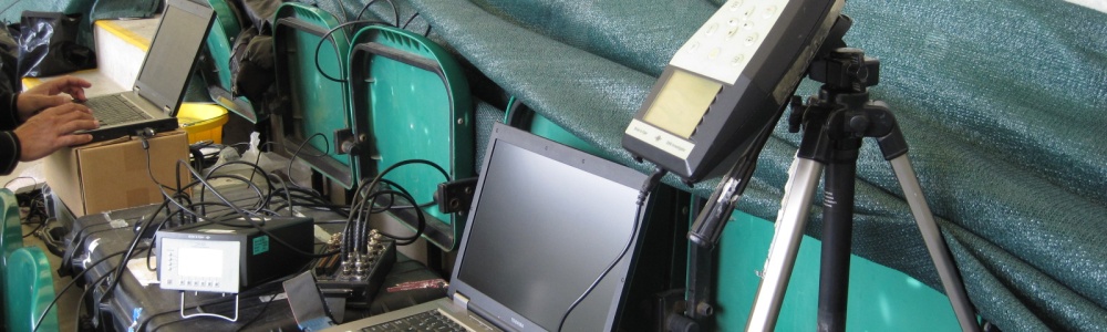
The channels were taken to a notebook computer through a 12 bit National Instruments AI-16E-4 'PCMCIA type' data acquisition card with a maximum sampling rate of 250kS/s. A portable BandK 4294 accelerometer calibrator was used to check calibration of the measurement system, which was verified before and after each survey. Plate 6.1 shows the equipment in the laboratory with the shake table facility to check performance of the multi-channel monitoring system.
Data was visualised and stored on site using a Virtual Instrument created by the Author using LabVIEW. Plate 6.2 shows the graphical program which created an eight channel recording instrument sampling data from 8 channels at 2560 samples per second per channel and storing 16 seconds of data at the users command. The sixteen seconds window was long enough to record most train pass-bys (see Figure 6.5). A longer duration of data could not be stored without causing a data overrun, unless the data was streamed directly to the hard disk, without screen display. It was judged that visual validation of all acquired data was paramount, allowing interaction to optimise signal to noise ratio, and resolution for the various set ups. Post processing was undertaken using MATLAB.
The measurement system was capable of recording vibration from 1Hz to 250Hz, representing a very adequate measurement range for train vibration. Measurement diagrams for the equipment set ups are shown in Figure 6.1. Whilst accelerometers themselves can have a wide dynamic range (e.g. 140dB for BandK type 4378), the usable dynamic range of the instrumentation chain is limited by the signal conditioner and the ADC, which in this case was limited to 50dB. The vibration measurement system was tested on a shake table and found to be linear over the range of levels anticipated. Noise measurements were taken using BandK type 2260 and type 2236 meters with a linear dynamic range of 80dB, which were calibrated using a BandK type 4220 pistonphone. Equipment was calibrated before and after each survey. Outputs were within 5% (0.4dB) of reference level traceable to National Standards, in amplitude and frequency.
6.5 Signal to Noise ratio
The signal of interest should exceed ‘noise’ which may either be from background vibration, a situation on which there is less experimenter control, and more significantly electrical noise in the measurement chain. A rule of thumb in Industry is that the signal to noise ratio should be 10dB (a factor of three). Error on the signal associated with this signal to noise ratio is 0.4dB (5%), shown in Figure 6.4. Appendix 6.1 describes an experiment to determine noise inherent within the instrumentation chain, which involved taking horizontal measurements on a pendulum in a quiet environment. Table 6.1 summarises the noise floor for the two groups of front ends used.
Table 6.1 Noise Floor of Instrumentation
|
Typical set up with 50m co-axial cable
Typical Amplifier Gain Settings > |
BandK2635/4378
(10,000) |
Kemo/BandK2646/4378
(500 gain) |
| Noise Floor (mm/s2 r.m.s.) |
|
|
Of the two groups of front end, one group (all BandK) provide a lower noise floor, representing the ideal instrumentation for the surveys, but could not be made available at all times. Therefore the second group of front end (Kemo/BandK) was used, but had a higher noise floor. Which front ends were used in the case study surveys is made clear in the relevant chapters. This noise can be reduced by appropriate site deployment.
Achieving the requisite signal to noise ratio from r.m.s. evaluation of a time history is not sufficient where spectral analysis is undertaken, and the requirement for an adequate signal to noise ratio should ideally be applied across the spectrum. A comparison of instrument noise floor with train vibration is shown in Figure 8.6 (all BandK front end) in Chapter 8, and Figure 9.5 (kemo/BandK front end) in Chapter 9.
6.6 Considerations for site deployment of Instrumentation
There are factors relating to good site practice; concerning coupling of sensors, deployment of multi-channel systems to reduce ground loops, triboelectric noise in cables and electromagnetic interference, which are discussed.
The sensors should be coupled to the structure or ground in a manner that achieves a faithful recording of the motion. Where brackets are necessary, they should be sized to ensure that resonant modes of the bracket with the coupled sensor are outside the frequency range of interest (see ISO4866:1990).
In multi-channel monitoring set ups there is a possibility that the accelerometer case and cable screen at various monitoring points in the ground and structure will not be at earth potential. This will allow a voltage difference to exist between the various points allowing charge to flow. This leads to ground loops which manifest in the form of a continuous ‘hum’, which effectively adds to the vibration output signal. This gives rise to false vibration level indications. Peaks arise at mains frequency, and its harmonics.
Precautions were taken to minimise this effect, which entailed earthing the instrumentation at one point and ensuring that this earth connection was reliable. The accelerometers were electrically insulated at their attachment points. This was inherently achieved by the insulating properties of the rapid araldite used to glue brackets to the concrete structures, and in addition a plastic sheet was placed between the magnet of the sensor and the steel bracket as an economical means of insulation. Trial measurements were taken until ground loop noise was minimised.
Electromagnetic Interference (EMI) can contribute to system noise. Typically due to signal cables laid near to cables carrying (a.c.) currents (current 'spikes' from fast switching circuits), or from sources such as an electrified railway and mobile phones. In practice co-axial (screened) cables give adequate protection.
In measurements using accelerometers, noise can arise due to motion of the microdot (miniature co-axial) cable from accelerometer to charge amplifier. This arises when a coaxial cable is subject to bending, compression or tension, where the screen may become momentarily separated from the dielectric at points along the cable. This causes local changes in capacitance and 'triboelectric' charges are formed, leading to noise. The cable was therefore where necessary secured to the structure to minimise motion, which often occurs in wind gusts or by the operator inadvertently disturbing the cables.
The Author positioned himself with the data recording instrumentation in a way that minimised cable lengths (signal loss) to all the sensors and to not allow his own movements to corrupt data acquired by local sensors. However as multi-channel recording was being undertaken, some sensors would inevitably be deployed in areas subject to vibration from occasional footfalls and site traffic, even though such measurements would be taken late at night.
As a result of possible data corruption, all the traces were examined by eye, and dispensed with where appropriate.
6.7 Post Processing for Spectral Representation
The spectral characteristics of a waveform may be represented in a variety of ways. If the waveform is simple the frequency can be deduced by counting the spacing of zero crossings. However, waveforms from train records are more complicated, requiring alternative methods to estimate the spectral characteristics.
In some cases bandpass filters, typically proportional bandwidth filters (e.g. third octave) can be used, but they do not provide adequate frequency resolution. An alternative method to determine the spectral characteristics is to use the Fourier series, which can be used to describe a periodic function of time. As the period 'T' becomes larger the frequency spacing D f between the Fourier coefficients becomes smaller, tending to zero as T® ¥ . In the limit, the Fourier series turns into a Fourier integral, and the Fourier coefficients become continuous functions of frequency called Fourier transforms. The spectral density is formally defined as the Fourier transform of the auto-correlation function, and the cross-spectral density between two random processes is defined as the Fourier transform of their cross-correlation function. It turns out that a discrete Fourier transform (DFT) can be readily obtained directly from a discrete time series, using the fast Fourier transform (FFT) algorithm (see Newland, 1993).
The statistical characteristics of the random process are assumed to be stationary (independent of time), and ergodic (in which any one sample completely represents the ensemble), but these assumptions are not entirely true for railway induced vibration (see section 6.9.4). In practical experiments that rely on a finite sample, errors are introduced into the measured spectrum. A consequence of analysing a finite record length is that sharp spectral lines (delta functions) that would otherwise arise from T ® ¥ actually smear out over a band of frequencies with a width of D f. In order to be able to resolve two nearby spectral peaks the record length must be long enough, to ensure the frequency resolution D f=1/T is smaller than the difference between nearby peaks.
The discrete Fourier transform of a time series does not provide spectral estimates localised in time, but refers to the record length analysed. Therefore we cannot identify the contribution to spectral estimates made by localised features in the time domain. An alternative is to utilise short-time Fourier Transforms, which localise features in the time domain using a shorter record length, which is repeated with overlapping windows over the time series. The overlap can be used to provide more equal weighting to the signal to compensate for the attenuating effect of a window on the ends of a record. Time resolution is restricted to this shorter record length, which for reasons of achieving frequency resolution and accuracy cannot be made too short. This underlies a fundamental uncertainty principle, where it is impossible to simultaneously achieve high resolution in time and frequency.
Instead of using sines and cosines to decompose a signal (Fourier analysis), an alternative orthogonal basis known as wavelets, which are local functions, can be used to determine the amplitudes of various frequency components at different times, and thereby identify the characteristics of local features (see Newland, 1993).
Spectral characteristics in this thesis are determined using third octave filters for noise and by the discrete Fourier transform for vibration.
The acquired waveforms required some basic post processing, involving removal of DC offsets, which can cause distortion of a spectrum, in the region of zero frequency. Trend removal may also be appropriate, but involves assumptions about the nature of the trend through the time history. It turned out that the data did not benefit from trend removal adjustments, other than by a very small amount at frequencies close to zero, and therefore this step was omitted. The time skew due to sequential sampling of 8 channels with the ADC was negligible, and therefore no corrections were made for this.
Duration of train pass-bys varied and were fortunately mostly adequately recorded using a 16 second window (limit on the pc based recording system for eight channels with real time display). The principle part of the train event could however in most cases be represented using a 12s window mostly centred on the event, as shown in Figure 6.5.
6.8 Transmissibility
When the spectra at two locations of a given parameter (e.g. acceleration) are compared as a ratio, it describes the amplification and reduction between the two points as a function of frequency. The transmissibility between two points, with random vibration signals x(t) and y(t), can be presented as two ratios, total transmissibility and direct transmissibility (terminology due to Newland and Hunt, 1991). These ratios involve the single sided auto spectra and cross spectra as follows, and are identical to the two sided spectral density (see Bendat and Piersol, 1986):-
Equations 6.1 and 6.2 are shown to be dimensionally correct on the right of the page by assuming the input x(t) is a force (N), and output y(t) a displacement (m), which yields receptance in both cases.
A simple proof of the above expressions can be taken from Bendat and Piersol (1986), reproduced here. Take a constant parameter linear system, with single input x(t) and single output y(t) shown in Diagram 6.1.
The output y(t) is obtained by the convolution integral in eqn.6.3, where h(t ) is the unit impulse response function.
For any pair of long but finite records of length T, eqn. 6.3 is equivalent to eqn.6.4 where X(f) and Y(f) are the finite Fourier transforms of x(t) and y(t) respectively, and H(f) is the frequency response function (transmissibility).
Y(f) = H(f)X(f)
Multiply both sides of eqn. 6.4 by the complex conjugate Y*(f)
Since Y*(f)=H*(f)X*(f)?
We obtain½ Y(f)ú 2 = ½ H(f)½ 2½ X(f)½ 2
Multiplying both sides of eqn. 6.4 by the complex conjugate X*(f) we obtain:
X*(f)Y(f) = H(f) ½ X(f)½ 2
![]()
![]() The single sided cross (Gxy) and auto (Gxx, Gyy) spectral density (f > 0) are defined as:
The single sided cross (Gxy) and auto (Gxx, Gyy) spectral density (f > 0) are defined as:
![]()
E[] denotes an averaging operation over index k, which represents the kth record of an ensemble of records of length T, which gives from eqn. 6.6 and eqn. 6.7:
Gyy(f) = ½ H(f)½ 2Gxx(f)
Gxy(f) = H(f) Gxx(f)
![]()
![]()
Eqn.6.11 is a real valued relation containing only the gain factor (c.f. Total transmissibility, proving eqn 6.1), whereas eqn. 6.12 is a complex valued relation providing the gain and phase (c.f. Direct Transmissibility, proving eqn 6.2). The total transmissibility compares the auto spectrum at one location, with the auto spectrum at another. The direct transmissibility on the other hand compares that part of the spectrum at one location, which is correlated to the other. It has been the Author’s preference to mainly examine disparity between total and direct transmissibilities to infer the degree of correlation, but this can also be seen by the coherence function (eqn. 6.13), which if used on total transmissibility recovers direct transmissibility (eqn. 6.14).
![]()
![]()
When total and direct transmissibilities are equal (g 2xy =1), it indicates that output signal is entirely correlated to input signal ![]() . However, in a real structure, the degree of correlation varies, as the output signal is influenced by vibration from the source of interest coming via other paths (e.g. neighbouring pile/columns) or due to 'noise' from other sources (e.g. building services) or due to non linearity of the system, and is therefore not totally correlated to the input
. However, in a real structure, the degree of correlation varies, as the output signal is influenced by vibration from the source of interest coming via other paths (e.g. neighbouring pile/columns) or due to 'noise' from other sources (e.g. building services) or due to non linearity of the system, and is therefore not totally correlated to the input ![]() .
.
Diagram 6.2 shows a real multi-input / output system, but which is characterised in the measurements by a single input / single output system. Tdirect can be used to assess the importance of a particular input or transmission path, and was used to calculate the unique characteristics between specific pairs of points. Tdirect could represent the behaviour of isolated column (A), when all the other inputs that arise are uncorrelated, but in reality there will be some correlation* of inputs from neighbouring columns and therefore detract from this idealised assumption.
6.9 Errors in Estimates
Different types or error can arise in the acquisition and processing of a measurement. There are errors associated with the instrumentation chain, comprising transducer, cable, amplifier, anti-alias filter and ADC (± 5% (0.4dB) from section 6.5). The signal of interest can be influenced by the instrumentation noise floor, although the error is small (0.4dB) when the signal exceeds this noise floor by 10dB (see section 6.4, Figure 6.4). Additional errors include a random error associated with analysing a finite length of record, and there may also be bias (systematic) errors in the estimate of spectral density.
6.9.1 Random and Bias Errors on Auto Spectra
The measured value of a random process can be expressed as a chi-squared random variable (c k 2) which is a sum of the squares of (k ) statistically independent Gaussian random variables. The random error of auto spectra (Gxx, Gyy) can be indicated by the ratio of the standard deviation to mean value, represented by eqn. 6.15, provided that the spectrum changes slowly in relation to D f=1/T (Bendat and Piersol, 1986). An increase in the equivalent number of statistical degrees of freedom (k ) (expressed by eqn. 6.16) improves statistical accuracy, and Figure 6.6 shows the benefits to be significant when (k ) is increased from a low value, although rate of benefit reduces.
The effective bandwidth of the spectral window may be approximated as Be@ 1/T, which gives a basic dilemma that increasing the record length 'T' does not improve accuracy (s /m@ 1 and k =2), because the spectral bandwidth reduces in proportion to 'T'. This dilemma does not arise with proportional bandwidth filters (e.g. third octave), because the filter bandwidth is fixed independently of 'T'.
Statistical accuracy can be improved by calculating the arithmetic average of (n) adjacent spectral estimates (2n+1), which has the following effect on the effective bandwidth and statistical accuracy (Newland, 1993).
We can see that an increase in statistical accuracy is achieved at the expense of frequency resolution.
Time series acquired using a given sampling rate for a given record length do not necessarily achieve a sequence length that is an integer power of 2, for which an efficient FFT algorithm can be used. Rather than reducing the record length to the nearest lower power of 2, zeros can be added to the time series to achieve the next higher power of 2. This has the benefit of implementing a faster FFT algorithm, but also has the benefit of improving frequency resolution. If 'T' represents the original record length, and 'TL' the record length after adding zeros, the effective bandwidth is clearly improved, Be@ (2n+1)/TL, where TL>T. But the statistical accuracy is reduced as k @ 2(2n+1)T/TL (Newland, 1993). As there are algorithms that can cope with time series that is not a power of 2, albeit more slowly, there is no incentive to add zeros, given that it reduces statistical reliability at the expense of improved frequency resolution.
When a hanning window is used to reduce spectral leakage, the effective spectral bandwidth (strictly: equivalent noise bandwidth) is actually Be=1.5/T (Harris, 1978). When (2n+1) spectral lines are averaged the effective bandwidth and the number of statistical degrees of freedom from eqn. 6.17 becomes:
Be=(2n+1.5)/T????k =3(2n+1)? ? eqn. 6.18(i,ii)
A total of 21 spectral lines were averaged to produce a smoothed spectral estimate, which was based upon achieving an effective bandwidth of 1.79Hz and achieving reasonable statistical accuracy based upon 63 statistical degrees of freedom. Figure 6.7 shows the raw and smoothed spectrum using a record length of 12 seconds. One effect of this averaging is to cause individual peaks in the spectrum to appear as rectangular peaks which have a flat top (21 lines wide º effective bandwidth), as seen from the mains peaks and harmonics in Figure 8.6 of Chapter 8. An explanation is evident by examining Figure 6.8, which shows that the effect of averaging a peak (tone in this example) using a linear averaging window. When a peak of constant value dominates, the average value is virtually constant, all the time the averaging window encompasses this peak. One way to avoid this feature is to only plot the magnitude at the centre frequency of the bandwidth, and do so for all neighbouring bandwidths across the spectrum. This is not an essential step and was therefore omitted.
The auto spectra estimates, with k =63dof, were calculated to lie within the range:
0.763Gxx < Gxx < 1.377Gxx ?(90% confidence) eqn. 6.19
If the spectrum changes quickly in relation to the effective bandwidth of the filter, then a bias error (systematic error) arises in the estimate of spectral density due to the finite frequency resolution used (see BS60068-2-64, 1995). Figure 6.8 shows an example of bias error, where the effective bandwidth causes a lower value estimate of the peak in the spectrum. Schmidt (1985) describes the form of this bias error for a hanning window, in eqn. 6.20(i), which is a function of the ratio of effective 'resolution' bandwidth Be and half power point bandwidth at resonance obtained from eqn. 6.20(ii).
For a typical base isolated building on coil springs, assume the smallest resonance frequency expected is 5Hz, with a critical damping ratio of 3%. This equates to a bandwidth for the resonant peak of Br = 0.3Hz, which requires an effective Bandwidth Be of 0.1Hz, to limit bias error to approximately -1dB. We have seen that to achieve a reasonable confidence level on the random error, it was necessary to average adjacent spectral lines, which has the effect of increasing the effective bandwidth (to 1.79Hz for T=12s and avg. of 21 lines). This contradicts requirement to reduce bias error and achieves poor frequency resolution, but spectral processing is a matter of compromises.
6.9.2 Random Error on Transmissibility
For a single input/single output system the random error (e r) on direct transmissibility is given by Bendat and Piersol (1993) as:
Where g xy2 = coherence (eqn.6.13), ½ g xy½ = +ve sqrt coherence, na = number of averages
This random error is a function of frequency, due to its dependence on the coherence function, reducing as coherence increases and with increasing number of averages (either across the ensemble or adjacent spectral lines). The random error on the total transmissibility is indicated by a similar expression and there are also bias errors (see Bendat and Piersol, 1993).
It is difficult to quote a single number random error value for transmissibility measurements, due to its dependence on coherence which will vary as a function of frequency, and between pairs of measurements in various parts of the structures. However in order to get a handle on this error we can recall the confidence limits on the individual auto spectra (eqn. 6.19) as follows:
![]()
The total transmissibility is therefore estimated to have a random tolerance of ± 3dB and believed to have 90% confidence, implying that measured changes above this range are statistically meaningful. It is clearly not appropriate to average the auto spectrum for different samples of train events across the ensemble, because there will inevitably be differences due to rolling stock, train speed and track used. It is however reasonable to average the transmissibility between two points, if it is assumed that it describes the effects of a linear system, where response is proportional to magnitude of excitation and the principle of superposition can be applied. The transmissibilities for the majority of set ups were therefore averaged using five train events and similarity allows one to deduce linear effects of the system with which we are interested.
6.9.3 Propagation delays
![]() Because measurement points are not always affected by the source at the same time, owing to varied proximity to the source, the propagation time delay (t ) effects would lead to errors. Schmidt (1985) indicates that this bias error is dependent upon the type of window used, and for a hanning window is of the form:
Because measurement points are not always affected by the source at the same time, owing to varied proximity to the source, the propagation time delay (t ) effects would lead to errors. Schmidt (1985) indicates that this bias error is dependent upon the type of window used, and for a hanning window is of the form:
The error is small when (time delay/record length (t / T))<0.1. This was significantly bettered in the case studies, since this ratio would imply a propagation time delay of up to 1.2s on a 12s record would be acceptable. Total transmissibility should be unaffected by propagation delay, as auto spectra are unaffected assuming a stationary random process.
6.9.4 Non-Stationary Data
When the statistical properties of data vary with time, the process is non-stationary, and it is not rigorous to obtain such properties by time averaging operations over a single record. Instead a collection of time history records measured under statistically equivalent conditions is required. A railway source is inevitably non-stationary (see Figure 6.9), and it is not possible to obtain records under statistically equivalent conditions (e.g. type of rolling stock, track used, or speed may be different between samples and not under the control of the experimenter).
![]()
![]() Bendat and Piersol (1993) describes a technique to establish optimum averaging time (To) and bandwidth (Bo), to minimise the total mean square error that comprises time resolution bias error, frequency resolution bias error and random error. These optimum parameters are reproduced in eqn. 6.24.
Bendat and Piersol (1993) describes a technique to establish optimum averaging time (To) and bandwidth (Bo), to minimise the total mean square error that comprises time resolution bias error, frequency resolution bias error and random error. These optimum parameters are reproduced in eqn. 6.24.
![]()
The time resolution bias error coefficient (CT(t)), is a function of time. It is suggested that the maximum value may be appropriate, and easily estimated for a non-stationary event that is half-sine in character (Bendat and Piersol, 1993), from eqn.6.25
Whilst a train event might be globally viewed as half-sine in character, in reality close up this is not the case (see Figure 6.10). This implies that the optimum parameters will vary according to the section of the record analysed. The optimum analysis parameters are a function of damping, and although one might assume a constant damping value, the derivation assumes that the modes are independent, and does not account for modal overlap that may arise in practise. If we set aside the above, we see that optimum averaging time and bandwidth are functions of frequency, where optimum averaging time is less sensitive to frequency than analysis bandwidth. By making an assumption that the event in Figure 6.10 is globally half-sine pulse in character, we estimate the optimum values for a system with 3% critical damping for three sets of frequency representing the range of major interest in Table 6.2.
Table 6.2 Optimum Analysis parameters for a system with 3% critical damping
|
|
|
|
|
|
|
|
|
|
|
|
|
|
|
Bendat and Piersol (1993) indicate that overall error is within 25% of the minimum value for averaging times and analysis bandwidths that lie within ± 50% of the optimum values derived by eqn. 6.24, implying a broad range is permitted. Actual analysis parameters adopted are (T=12s, Be=1.79Hz). Even allowing for the broad range it would be difficult to minimise the error for the entire frequency range of interest. We will therefore suffer a time resolution bias error and a frequency resolution bias error that increases as lower frequencies are analysed.
Given the multitude of train time history records to be analysed and immense variability in non-stationary characteristics that exist, it is not realistic to meet optimum values for each analysis. The best approach was therefore to select part of the record that is quasi-stationary. This may conflict with the requirement to obtain a record long enough to minimise random error, when train pass-by event is short. Given a hanning window tapers the ends of the record, it was the Author's opinion that the record length chosen for analysis could as a compromise be extended beyond the ideal quasi-stationary part, to increase record length to reduce random error.
Conclusions
This chapter has shown the basic yet important procedures to ensure good quality data is acquired and described how to improve statistical confidence in the spectral estimates. The vibration caused by train pass-bys, are by their nature discrete events and the limited record length available makes the trade off between statistical accuracy and frequency resolution more acute. Whilst spectral averages across the ensemble is inappropriate given the inherent differences in train events, averages of transmissibility between two points are appropriate. This is because transmissibility describes the effects of a dynamic system, which is assumed to be linear even though the input and output to the system may be described as random processes.