
Projects
Industrial Sponsorship
Dynamic Performance Investigation of Base Isolated Structures
By Ather K. Sharif
7.1 Introduction
This chapter describes an experiment to examine the dynamic performance of a base isolated structure. The experiment was devised around the requirements of a developer to produce very high quality housing on a site directly above an underground railway. The site in Swiss Cottage, London, consisted of two proposed four-storey detached houses. A site plan in Figure 7.1(a) shows the outline of the two buildings in relation to the estimated alignment of the tunnel. The tunnel is used by British Rail for Intercity train movements between Euston Station and the North-West. The tunnel depth was not known accurately, but estimated from record drawings to be some 8m below ground level to the crown, which is shown in section in Figure 7.1(b).
The developer's specification called for noise and vibration to remain totally imperceptible, with isolation measures optimised as much as technically possible. For a relatively small development, the technical design requirements to achieve the high specification would have been onerous on the developer. As a result the design became a research exercise undertaken by the Author which was substantially subsidised by Civil Engineering Dynamics Ltd, the sponsors of this PhD. The design and construction period for this project spanned 2½ years from 1995.
The experimental investigation involved measurements on a test room in its un-isolated condition, which was then jacked and lowered onto three types of isolators; GERB coil springs, BTR natural rubber bearings and TICO synthetic rubber bearings. The measurements were undertaken in a way to provide the actual insertion loss for base isolation. Measurements were also repeated in the completed building, both in its un-isolated, and then uniquely in its isolated condition, where the Author conceived that the steel coil isolators be pre-stressed to allow them to be used to raise the building itself, allowing an economical means for the test.
7.2 Ground Conditions
Trial pits were dug by a Contractor to a depth of 1.5m below existing ground level, with hand auger boreholes (50mm dia) sunk through the base of the trial pits to a depth of 6m below existing ground level. This revealed made ground, overlying very stiff to hard brown mottled fissured silty clay. This London clay was found from a depth of 0.6-1.0m downwards. The concrete raft for the building was to be cast in the London clay, through which the tunnel runs. Details of the soil borehole log are shown in Figure 7.1(c). Clay soil properties are taken as the following approximate values: bulk density 2000kg/m3 , shear wave velocity 190m/s, compression p wave velocity 730m/s, and Poisson ratio of 0.46 (see Sharif, 1999).
7.3 The Proposed Structure
A concrete raft 450mm deep was to be constructed across the footprint of the two buildings shown in Figure 7.2(a). One building was to be constructed directly over the tunnel, Building 'A', with 'Building B' to one side of the tunnel. From a dynamics point of view it was desirable to have the rafts for each building constructed separately to minimise effective transmission of vibration. However for geotechnical reasons, to limit pressures on the tunnel below, a single raft was deemed necessary. The building has a basement and effectively provides four storeys, with the upper storey built inside the roof space. The Architect's proposed rear elevation is shown in Figure 7.3(a), with the Basement plan in Figure 7.3(b) and a cross section through the building in Figure 7.3(c). Plate 7.2 shows a rear view of Building 'A' completed.
Building construction was originally conceived to be in load bearing brick with reinforced concrete floors. Research by the Author on other case studies, reported in subsequent Chapters of this thesis, and the work of Newland (1989), Grootenhuis (1989) and Cryer (1994) identified a risk of resonant modes of the structure negating the isolation benefits predicted from rigid body models. To minimise these resonant effects occurring within the dominant spectra in the ground, analysis dictated that the structure should be stiffened to approach 'the ideal' rigid body model. The use of brickwork and concrete materials was expected to provide adequate damping to limit response at inevitable resonances. It was also desirable to increase mass as much as practical to reduce vibration response of elements above their resonance frequency (see Chapter 5).
A site restriction on building height and depth of excavation limited the available space for any isolators (to a maximum depth of 200mm) and the size of the ring beam to the walls (to a maximum depth of 300mm).
Finite element models of the structure, taking due consideration of the large perforations in the fabric for door and window openings, indicated that the external walls should be made of reinforced concrete for the full height of the building, with a cavity and external finishing in facing brick to increase stiffness of the shell (see Sharif, 1999).
The thickness of these outer walls from vibration control considerations was specified as 200mm concrete, with a 75mm cavity and 100mm high density facing brick (without voids). An exception was the rear wall, at basement level. This comprised the large patio door openings, and was therefore specified with a thicker 300mm concrete wall, but with the same cavity and brickwork. Internal cross walls in the basement were similarly specified as 300mm thick in reinforced concrete. The central spine wall running front to back of the site, was set to 300mm width in concrete for the full height of the building. The north external wall at basement level, turned out to be wider, although for architectural rather than dynamic considerations.
Floor thickness was specified, based upon calculation of first mode natural frequencies, which were targeted to be (at 20Hz to 30Hz) just below the dominant peaks in the ground spectrum. To help achieve this, screed was to be added to the floor, but decoupled using bitumen paint. The proposed use of bitumen paint in this way was to allow the added mass of the screed to force the natural frequency to come down, without the screed adding to the stiffness of the floor. (In the event this decoupling proved to be unnecessary, and the bitumen paint was not applied).
7.4 Test Room
As no data existed on the insertion loss for base isolated structures, it was desirable to validate the actual benefits of base isolation and identify any weakness in performance that would need to be addressed in the final design.
It was also necessary to validate the choice of target natural frequencies from available isolators. The isolators under consideration, with their respective target vertical natural frequencies were as follows: -
Table 7.1 Isolator Target Natural Frequencies'
| Isolator | Target Vertical Natural Frequency |
| GERB Steel Helical |
|
| BTR Natural Rubber |
|
| TICO Synthetic Rubber |
|
A test room was therefore built on the raft for a series of detailed measurements. It was initially mounted on concrete blocks, to represent the un-isolated case. It was then jacked and lowered on to three different sets of isolators to represent the base isolated cases. Plate 7.1 shows a general view of the concrete test room with a view looking in a north-easterly direction across the site.
The test room was conceived to be one of the ground floor rooms to the final building. This allowed it to be incorporated into the final construction, thereby avoiding the need to construct a separate test room, that would be subsequently demolished and therefore wasteful. Figure 7.3(a) shows the Architect's rear elevation of Building 'A' which is directly above the tunnel. The extent of the test room is marked on this drawing, and Figure 7.2(b) shows a plan of the test room, which is seen to form one corner room to Building 'A'. (This room is the eventual "Family Room" of Figure 7.3(b))
The test room is a reinforced concrete box with openings for doors and windows. The wall thicknesses are shown in Figure 7.2(b). The ground floor and first floor of the test room were 225mm thick in reinforced concrete and actually become the basement and ground floor respectively for the final building. The test room mass was about 80 tonnes, with the final building 665 tonnes, both unfactored (dead loads).
The test room was to be supported at eight points shown in Figure 7.2(b) which also shows the temporary jacking points. The test room was initially cast on soffit shuttering made up of two layers of 100mm blockwork placed on a compacted layer of sand, 25mm thick. When the test room was completed and the concrete had reached adequate strength, the test room was raised using hydraulic jacks to facilitate removal of the temporary block work and sand.
The test room was then lowered onto concrete blocks at the eight support points to represent the un-isolated situation. These concrete blocks were stacked two- high at each support location. This stacking was required owing to the starting height of the void, and the requirement to raise the test room to accommodate the height of isolator units, with the minimum of intermediate jacking operations. This became necessary as there was a limit on the displacement of the jack piston (50 mm), after which it required resetting.
When the series of measurements for the test room on blocks was completed, the test room was jacked and the isolators were placed at the same position as the concrete blocks. The test room was then lowered for the next series of measurements. This was repeated until the three sets of isolators had been tested in turn.
To allow meaningful internal noise measurements, window and door openings were boarded up with plywood. The rear patio door openings were fitted with temporary glass sliding doors. Any air gaps were filled with foam. The trap door in the ground floor, required for future access to the isolators, was also boarded over in plywood.
7.5 Test Room Supports
The test room was initially supported on concrete blocks and then on three sets of isolators shown in Plate 7.3, with Plate 7.4 showing an internal view for the make up of the GERB coil spring isolators. Plate 7.1 shows the test room supported on GERB coil spring units (inset to Plate 7.1 shows the test room on concrete blocks).
7.5.1 Concrete Blocks: 'Idealised Rigid' Un-Isolated Case
8No 200mm wide x 400mm long x 175mm deep plus 8 No 100mm deep (Characteristic 28 day strength of 40N/mm2).
The concrete blocks under the test room had a low compressive stress of 1.2N/mm2.
A finite element model of the concrete blocks stacked as a pair in series was analysed by the Author (Sharif, 1999) and reported to have an axial stiffness of 9.3 x 10⁹N/m, and with the test room mass exhibits a first mode natural frequency of 151Hz. In practice the blocks themselves are supported by the raft on a 'soil spring' which would lower this frequency. They therefore do not provide an ideal rigid case although they resemble a structure supported at points, such as by columns on a grid.
It was originally conceived that the blocks should be attached to the raft with a thin mortar bed, and likewise a thin mortar bed was required between the blocks and the soffit of the test room to ensure good coupling. Unfortunately for programme/cost reasons (time for mortar to set, and additional effort in breaking joints), this request could not be accommodated by the Contractor.
7.5.2 GERB Coil Springs: Target Natural Frequency 4.5Hz
8No GERB GPNV-2.0-3617/20K 295mm tall, with plan dimensions of 440mm x 200mm
Compressive stress on the bearing face is not a relevant parameter for steel isolator units, given that permissible stresses are limited more by concrete strength. Load on the steel coil springs is however a design consideration in the context of stability.
The unit consists of two coils made from a wire diameter of 36mm and an outside coil diameter of 151mm, with the lower unit filled a third full with a viscous fluid providing 3% critical damping (GERB, 1996). The coil is in contact with the housing via a steel washer which is in contact with a neoprene sleeve/washer, and glass paper washers. The make up of this coil unit is shown in Plate 7.4 with further details given in Appendix 7.1. It is possible to nest smaller diameter coil springs (wire diameter 17mm / od 69mm), inside the principle coils to increase the stiffness, but this was not required for the test room.
7.5.3 BTR Natural Rubber Bearings: Target Natural Frequency 8Hz
16 No BTR AE1320 150mm x 150mm x 80mm thick
Compressive stress on the rubber bearings was 2.2 N/mm2 (The maximum permissible value depends upon stability requirements, and the need to avoid long term degradation (see Thomas, 1982)).
This unit is a laminated bearing containing three steel plates. The manufacturers state the damping achieved for their natural rubber bearings is 3-5% of critical represented as viscous type (Andre, 1998). These were placed in pairs at the eight support points. Owing to the height of the void, these were parked onto a single concrete block. The stiffness of the concrete block would act in series with the stiffness of the BTR bearing. But this does not materially alter the overall stiffness of the support bearing.
7.5.4 TICO Synthetic Rubber Bearings : Target Natural Frequency 12Hz
8 No TICO CV/M 300mm x 300mm x 50mm thick
The compressive stress on the TICO bearings was 1.1 N/mm2 which would achieve the target natural frequency, and was within the permissible range of 1N/mm2 to 1.4 N/mm2 for this particular product (see TICO prom lit).
This unit is made from neoprene impregnated with cellular particles. The manufacturers state the damping for this synthetic rubber bearing is 6-8% critical represented as viscous type (TIFLEX, 1998). Owing to the height of the void these were each placed on concrete blocks, with two concrete blocks laid side by side to achieve the bearing area for this larger unit in plan. Again, the concrete block used in series with this TICO bearing would not materially alter the overall stiffness of the support.
7.6 Instrumentation
Two set ups were used for vibration monitoring. Either an eight channel or four channel PC based monitoring system, as described in Chapter 6. Of the monitoring systems used (mostly Kemo/BandK), a more expensive lower noise configuration (all BandK) could be used on some occasions, and is noted accordingly in the results and discussion. Whilst it was desirable to use a given configuration of equipment for every set up, using equipment with the highest sensitivity and lowest noise floor where appropriate, cost was a major issue. The Author therefore was required to make the best use of whatever resource was available at the lowest cost. Figure 7.2(b) shows the accelerometer monitoring positions, labelled 1-8 when the eight channel system was used, or locations 1- 4, when the four channel system was used.
Noise monitoring was undertaken in the room using two Bruel and Kjær noise meters: a 2260 third octave real time analyser and a 2236E noise meter. These were calibrated using a Bruel and Kjær 4231 calibrator.
The noise meters provided maximum Sound Pressure Level (LAmax) and Equivalent Continuous Levels (LAeqs ) in dBA, over 1 second intervals. Bruel and Kjaer 2260 meter also recorded 1 second third octave spectra. Microphones were placed in the centre and off centre positions, in the room, shown in Figure 7.2(b), at a height of 1.25m. Noise meters were set to 'fast' time response (terminology: Chapter 3; ISO1996 Part 1, 1982).
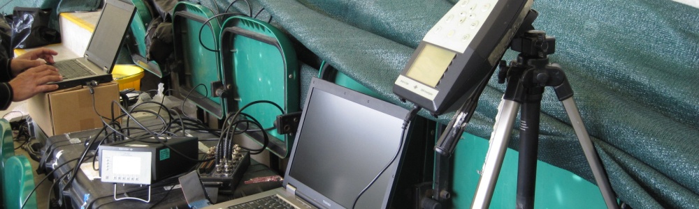
Plate 7.5 shows the instruments set up in the test room where the Author was also seated during the measurements. Accelerometers were attached using magnets to a steel bracket that was glued to the structure using rapid hardening Araldite.
7.7 Strategy to determine Insertion Loss for Base Isolation
To establish the insertion loss due to base isolation, comparative measurements were required between a 'free-field' measurement location, and the structure with its various supports. It was assumed that the dynamic characteristics of the 'free-field' measurement location would remain constant, and therefore changes in the comparisons with this datum could be attributed to the effects of alternative supports.
Diagram 7.1 shows a schematic section (E-W), indicating the relative position of the 'free-field' test block and raft with the tunnel below. [D1] indicates transmissibility from the test block to the raft (see Chapter 6 for definition).
Un-isolated Case
Diagram 7.2
D2 - D1 = effect of loading raft "Building without Springs" eqn. 7.1
D3 - D1 = effect of Building on concrete blocks eqn. 7.2
D3 - D2 = effect of "non-ideal" rigid blocks eqn. 7.3
Isolated Case
Diagram 7.3
D4 - D1 = effect of Building with springs eqn. 7.4
Benefit of base isolation =
{effect of building with springs} - {effect of building without springs}
[D4 - D1] - [D3 - D1] eqn. 7.5
or
[D4 - D1] [D2 - D1] eqn. 7.6
From which, D1 cancels, giving: -
Benefit of base isolation = [D4 – D3] eqn.7.7
or
= [D4 – D2] eqn. 7.8
depending upon which reference [D3] or [D2] is used for the un-isolated case.
The benefit of base isolation [D4 - D3] or [D4 - D2], is considered to be the 'true' insertion loss for base isolation, where if the concrete blocks were 'ideally rigid', D3 and D2 would be identical.
Now, it is evident from diagram 7.3 that :-
D4 = D5 + D6 eqn. 7.9?
Therefore, substituting eqn. 7.9 into eqn. 7.8, we get: -
Insertion loss for base isolation = D6 + D5 - D2 eqn. 7.10
where [D5 - D2] = difference in the raft response loaded through
mass on springs or blocks eqn. 7.11
Therefore, [D6] might be used to describe insertion loss for base isolation, if [D5 - D2], the difference in response of raft loaded via blocks or springs is small.
Experimental Assumptions
- The trains are clearly non-stationary events, yet we have to analyse them using random process theory as though they were stationary events (see Chapter 6).
- [D1] is a measure of the transmissibility from the test block to the raft, which can be accounted for by a number of factors:-
- The dynamic characteristics of the raft compared to the test block; indicating both differences in local characteristics (dynamics of test block /raft with the soil) and non-local characteristics (attenuation due to intervening ground)?
Local characteristics:
Ideally the test block should resemble 'free-field' conditions, but in reality its mass on the soil spring represents a system which has its own resonance characteristics.
The test block mass on the soil spring exhibits a set of values for mass, stiffness and damping, according to the mode of oscillation, represented as: -
Diagram 7.4
The raft differs from the test block in its mass, stiffness and damping, which again vary according to mode of oscillation, represented as: -
Diagram 7.5
The resulting difference in natural frequency and damping between test block and raft of both rigid body and flexural modes affects their relative response to the train vibration source. The effects of any differences are assumed to be constant between surveys.
Non-Local Characteristics
Attenuation characteristics of intervening ground which are assumed to be constant.
(ii)?The test block and raft are not at identical distances from the tunnel (see Diagram 7.1). The exact values are not known, as there is no accurate information on the tunnel alignment. Therefore whilst distance to the moving train source varies at a given measurement location, the two locations are at different distances to start with, which is a constant.
- If the vibration from the train is dominated by the wheels traversing a defect in the track, the distance of these defects from the test block and the raft will not be the same (see Diagram 7.1). This affects not only the magnitude but also the temporal position of the peaks. Fortunately, one of the disadvantages of Fourier analysis used in the auto spectrum estimates, whereby it is unable to identify the point in the lifetime of a particular feature, turns out to be useful. It means that the spectral estimate is largely insensitive to the temporal position of the peaks, although it will be sensitive to magnitude difference of the peaks.
- Ground vibration waves will interact with the test block and raft according to how the wavelengths compare with the dimensions of the structure, and the impedance mismatch. The difference in the relation of wavelengths with the test block and raft foundation can alter wave reflection, transmission and diffraction in a frequency dependent way. The difference in impedance between the two cases may not be immediately obvious, given that the concrete materials for the test block and raft should have identical acoustic impedance (for concrete acoustic impedance r c=8x10⁶ kg/m2s, see Hall, 1987). Yet the mechanical impedance is affected by the resonant characteristics that arise from the structural use of the material. Clearly a large block of concrete will offer different impedance mismatch with soil, compared to a thin slab of concrete on the same soil. These relative ‘scale’ effects are however assumed to be constant between surveys.
Differences in train events (rolling stock, speed, track used) could affect transmissibilities. It is assumed that they are independent of train event.
- Non-linearity (characteristics that vary with level of strain). The environment is assumed to be linear.
Items (i) to (vi) are collectively referred to as difference [D1] which therefore represents the effect of the raft construction in comparison to the test block, but includes factors unrelated to the raft itself. As we cannot distinguish between the individual factors, we refer to [D1] as the idealised case of the effect of 'free-field to raft'. The analysis is based upon the mean result of 5 train pass-bys.
It becomes an experimental assumption that any changes that arise on the mean transmissibility results in subsequent surveys occur due to the effect of change in support being investigated (un-isolated to isolated condition of support).
We could not for practical reasons in this series of test achieve monolithic construction with the raft for the un-isolated case, as we would need to be able to raise the building easily to introduce the isolators, and have an air gap everywhere else. It was therefore assumed that the building supported on concrete blocks could represent the un-isolated condition.
The mounting of the building onto concrete blocks should largely allow the inertia effect of the building to arise in the same way that it would arise with traditional monolithic construction, up to 100Hz, which is well below the resonant frequency of the blocks (see section 7.5.1). However the discrete supports would not be able to recreate the stiffening effect that a traditional building structure would impose on the raft. The possible increase in damping afforded to the raft by the building is likely to be insignificant, given that a raft foundation embedded in the soil is so heavily damped, that the damping that is available in a building (usually represented as 5% critical) is unlikely to be a significant contributor. Therefore any differences in damping effect afforded to the foundation between monolithic construction and that on blocks becomes more negligible. (The same argument does not however apply in the effect that soil damping can have on the damping of the building, which can be significant.)
We can summarise that whilst it is assumed that the building on concrete blocks represents the un-isolated condition, it will not recreate the stiffening effect of a building upon a foundation and vice versa.
In this experiment, the effect of loading the raft with the test room or final building is referred to as the ‘mass effect’ on the raft, although changes that may arise due to alterations in stiffness and damping are ignored.
7.7.2 Achieving 'free-field' condition for datum measurement
A 'free-field' measurement condition was required to allow measurements at other locations to be referred to this as a datum. If the coupling of the sensor to the soil introduced artificial characteristics, any reference to this datum would show not just the characteristics of the system being investigated (for example the isolated building), but also inevitably the characteristics of the datum measurement. Whilst it was assumed that the characteristics of the datum situation should be a constant in any subsequent comparisons, it was still desirable to reduce the magnitude of any artificial characteristics of the datum measurement.
It is therefore important that the nature of the coupling of the sensor to the ground should faithfully reproduce the motion of the ground (see Skipp, 1984). However, there are practical constraints.
Firstly the 'free-field' sensor would need to be orientated in 3 directions, necessitating a bracket with three orthogonal faces. The triangular bracket, measuring some 60mm, could not be placed directly on the exposed clay strata. This is because the small dimensions of the sensor would make it sensitive to local characteristics of the clay, and it would be impossible to replicate the fixing over the long period of the project, with a surface also exposed to weathering. The sensors could be buried and back-filled with soil to embed them (Jakobsen, 1987), but again this would be sensitive to changes in 'workmanship' between site visits. It was therefore necessary to provide a firm contact surface, which itself was well coupled to the clay, and allow a reproducible method of coupling the sensor to the block. A concrete block, nominally 1m square and 0.5m thick was therefore cast with its formation level 1.5m below ground level in the clay (to match the proposed formation level of the raft).
7.7.3 Test Block Dynamic Characteristics
Vertical response of the test block to an impact on the ground is shown in Figure 7.4(a), where the free decay part should indicate its natural frequency, although it is well damped. We can alternatively examine the auto spectrum estimate shown in trace (b), which shows predominant response at around 25Hz, 50Hz, and 85Hz. These are not all necessarily the resonance frequencies of the test block as will be explained.
A theoretical analysis of the test block was undertaken using the method of Novak (see Novak and Beredugo, 1972; Novak et al, 1993). This consists of modelling the rectangular rigid footing on an elastic halfspace, with the embedment analysed as a series of infinitely thin horizontal soil layers extending to infinity, where each layer behaves independently of others. It is reasonable to assume that the soil below the footing is a halfspace, provided the strata depth is greater than 5 times the equivalent footing radius. For this assumption to be true, we require a minimum strata depth of 3.38m, which is satisfied, for the tunnel structure, which is at a depth of some 6.5m below the base of the footing. The method of Novak is incorporated into a computer program Dyna4, which was run on a PC. The program required the total mass and mass moments of inertia of the rectangular block, as well as the soil dynamic properties. The test block as built measured 1.1m x 1.3m x 0.5m deep (embedded) and soil properties for the site are given in section 7.2 (also Appendix 5.1). An arbitrary force and couple was applied in all six degrees of freedom, in the frequency range 0 to 200Hz.
Figure 7.5(a) (big crosses) shows the vertical receptance of the test block, where response looks heavily damped, with no resonance features visible. It should be noted that the effective damping is largely due to radiation damping, rather than material damping (a low value of 5% critical for London clay was assumed).
To emphasise the resonance characteristics of the block, the Dyna4 program allows one to reduce the actual computed damping value to exaggerate the response. In this case calculated damping values were reduced by a half. The vertical receptance of the test block is shown in Figure 7.5(a), compare crosses (actual damping) and circles (reduced damping). The response obtained using a reduced level of damping indicates a potential resonance at around 60Hz.
It is recognised that whilst the test block is quite thick in relation to its plan dimensions, it may still however behave like a flexible mat. To investigate this, it was modelled as a flexible mat foundation using Dyna4, but could only be modelled on the surface, as the program cannot include embedment for this case.
We can firstly compare the effect of this program restriction by comparing the vertical receptance of a rigid block that is embedded with that obtained for a rigid block on the surface. Figure 7.5(a) (dotted line) shows that the rigid block on the surface is more easily excited and displays a resonance frequency that can be discerned around 40Hz.
The effect of modelling the test block as a flexible mat on the surface is also shown (meshed with a 9x9 grid of node points), where a vertical harmonic load was applied on the central node. It should be noted that soil material damping is ignored in the mat foundation analysis, as for mats it is considered that radiation damping into the halfspace is dominant. Whereas, the rigid mass model incorporates the effect of material damping as well. The result shows that the test block if modelled in more detail, as a flexible mat, does in fact exhibit higher receptance, and the character of the result is broadly similar to that of the rigid block modelled on the surface.
We can therefore conclude that a resonance frequency for the test block would lie somewhere between 40Hz and 60Hz. This therefore would explain the peak in the impact response at around 50Hz (see Figure 7.4(b)). Yet there were additional peaks at around 25Hz and 85Hz.
Given that the impact mass itself could oscillate on the ground at its own natural frequency, and generate a wave train that could drive the test block, a similar theoretical analysis was undertaken for this situation. Figure 7.5(b) shows that the impact mass (168kg and 0.45m dia.) when modelled as a rigid block on the surface exhibits a resonant frequency around 100Hz which would appear to explain the measured peak in the test block response around 85Hz.
To examine the lower peak around 25Hz, we can examine if the raft itself could have responded to the impact, generating a wave train at this frequency. The raft was modelled as a flexible rectangular mat 14m x 28m, with a mesh of nodes at 0.5m intervals. These nodes could be used to apply loads and extract vertical response. In reality the raft was embedded below ground level, with retaining walls along all four boundaries as shown in section in Figure 7.3(c). The height of the retaining walls varied from 1m to 2.4m. The retaining walls would clearly stiffen the edges of the mat. However, the Dyna4 program could not accommodate these details.
The raft was analysed in three conditions. Firstly unloaded, then loaded with the mass of the test room distributed over eight support points, and then loaded with full mass of the building distributed as line loads in accordance with wall layout in Figure 7.3(b).
We need at this point only concern ourselves with the behaviour of the raft when it was loaded with the test room (shown as the dashed line in Figure 7.28(a)), as it is under these circumstances to which the impact test result shown in Figure 7.4 refers to. This analysis of the raft does not indicate resonant frequencies around 25Hz.
Whilst the analysis has assumed that an elastic half space is a reasonable assumption, in reality the crown of the railway tunnel is at around 6m below the soffit of the test block. Using the wave propagation velocities (v) quoted in section 7.2, we can predict standing waves (nv/2L) that could arise between the test block and the crown of the tunnel (L @ 6m), at (n) integer multiples above 16Hz for shear waves and 61Hz for P waves. These do not explain the vertical response of the test block at around 25Hz. It may be that the arch of the tunnel itself might exhibit this frequency, or that the topsoil and fill of 1.5m thickness over the London clay, might exhibit a pseudo natural frequency of this strata.
The peak in the response of the test block at around 25Hz has not been explained, however it is reasonably certain that this is not a resonance frequency of the test block. We have identified possible reasons for the peak in the measured spectrum at 85Hz, being associated with the impact source or due to p wave reflection between test block and tunnel structure. We are therefore left with a peak in the measured spectrum of around 50Hz, which was shown to be a natural frequency of the test block on a soil spring. The concrete block is of a size that it does not itself exhibit flexing or axial modes within the frequency range of interest. The assumption that the test block is a ‘free-field’ measurement condition is not strictly met, but fortunately the fact that it is a highly damped, means that a resonance effect is less pronounced than might otherwise have been. The test block will also reflect, admit, and diffract ground vibration in a way that is frequency dependent. These features in the response of the block were assumed to be constant between measurement situations. The test block is therefore referred to as a ‘free-field’ datum, against which the response of the building with its various supports could be evaluated.
7.8 Test Block to Unloaded Raft [D1]
Measurements were taken on the 'free-field' test block and the raft, when it was vacant of any structures. These results have been reported by the Author (Sharif, 1999), which indicated that the vertical response of the raft was comparable to the vertical response of the test block, although in the horizontal plane the raft response was much less, owing to its larger stiffness in this plane.
7.9 Test Room Measurement Procedure
All measurements were taken in the evening when the Contractor had finished work on site. Noise was measured in the centre and off-centre position inside the test room. Vibration measurements were taken in three orthogonal directions, being vertical and two in the horizontal plane, being tangential and longitudinal. One measurement location was on the test block, with others on the raft and the test room itself. Figure 7.2(b) shows the measurement locations labelled 1 to 8, described as follows:-
- Channel 1 on the test block
- Channel 2 on the raft
- Channel 3 on the ground floor in one corner of the test room, directly above channel 2 on the raft (representing measurements above and below the rigid blocks/isolators).
- Channel 4 on the centre of the first floor of the test room
- Channels 5 to 7 on the ground floor in the other three corners of the test room.
- Channel 8 is at another location on the raft.
A concrete mass (168kg) formed as a cylindrical block, 450mm in diameter, 440mm in height, was dropped or swung through various fall heights to excite the ground and the test room. This was used to identify response characteristics of the structure, and to see if impact tests could be used to simulate a rail source for a small structure.
7.10 Test Room on Concrete Blocks
This section describes measurements with the test room mounted on concrete blocks, intended to represent the un-isolated case. Figure 7.6 shows time histories of vertical measurements for a train event. A small delay in the start of the train event arises for measurements on the raft and the test room compared to the test block. This delay is attributed to this train approaching the test block first as it traverses the site. The magnitude of the event alters owing to the varying distance of the train as it traverses beneath the site. The wave form shows a higher intensity part to the event which could be due to the heavier locomotive of the train, compared to lower levels pertaining to the lighter carriages. It is seen that the test block levels, Ch1 are reduced into the raft Ch2. These are then slightly increased into the corner of the test room Ch3. These corner wall levels are then magnified into the first floor of the test room, Ch4. The net result is that the first floor midspan levels are in fact higher than the 'free-field' test block levels by a factor of about 2 times.
Figure 7.7 shows an estimate of the auto spectrum for measurements on the test block and raft. The spectrum is strongest between 30Hz and 90Hz, with substantially lower levels below and above this frequency range.
Figure 7.8(a) shows the coherence between measurements on the 'free-field' test block and the raft. The coherence is generally greater at low frequencies and reduces at higher frequencies. Figure 7.8(b) shows the coherence between two measurement points on the raft (between Ch2 and Ch8, see Figure 2(b)). This again shows greater coherence at low frequencies, which reduces at higher frequencies. If the raft were truly rigid, it would move as a whole in unison, and we would obtain a higher degree of coherence between measurement points on it. However, the fact that there is a low coherence, indicates that it is a flexible structure, where different parts are excited in an incoherent way.
The total transmissibility to four corners of the test room can be compared in Figure 7.9, along with the transmissibility to two locations on the raft itself. This shows that the raft and the test room on blocks exhibit a similar transmissibility at low frequencies, up to 50Hz, with a greater departure occurring at higher frequencies.
The transmissibilities were established for 5 train events, with the mean transmissibility to the raft and the corner of the test room on blocks compared in Figure 7.10. The difference in motion between the loaded raft and the "idealised" rigidly supported test room occurs because the concrete blocks are not actually rigid. At low frequencies the test room and the raft largely move as one, but at higher frequencies, the discretely supported test room on concrete blocks, enjoys some isolation from the higher frequencies. This implies that a discontinuous construction using discrete supports (concrete blocks) offers some benefit at high audio frequencies.
In traditional, un-isolated construction, the building would be cast monolithically with the foundations, in this case the raft. A more realistic assessment of performance can therefore be made by comparison with transmissibility to the raft, when it was loaded with the test room on blocks, as the un-isolated case. The only disadvantage is that comparisons between transmissibility to test room on coils and on blocks do not now refer to the exact same location.
7.11 Test Room on GERB Coil Springs
This section describes the series of measurements when the test room was on GERB coil springs, representing one case for isolation with a target vertical natural frequency of 4.5Hz. Figure 7.11 shows the time history for vertical measurements for a train event. In this case, the levels of vibration at the four corners of the test room and the first floor are so attenuated that vibration is hardly visible when viewed at the same scale as the raft and 'free-field' test block.
The total transmissibilities were obtained for 5 train events, shown in Figure 7.12. This shows that up to 100Hz the total transmissibility is largely independent of train events. This confirms that it was the system characteristics that were being obtained which are independent of the individual train characteristics.
There is however greater difference in the results above 100Hz, where the curves also ramp. It is proposed that the ramp arises because the source levels from the train above 100Hz were so low, and the efficiency of the isolation was so great, that 'noise' at one location was being compared with 'noise' at another location.
In order to investigate this more fully, a more expensive lower noise kit was used for additional measurements (see Chapter 6). The discrepancy between the two measurement systems is shown in Figure 7.13, which compares the mean total transmissibilities for the two measurement systems. Using instruments which have a 'low noise floor' the ramp in the transmissibility plots that were seen, can be reduced. The Author has reported that the scatter in the total transmissibility above 100Hz for different train events was also reduced using the lower noise kit (Sharif, 1999).
The test room on GERB coil springs has shown isolation above the rigid body natural frequencies. However, there are reduced attenuation peaks, which are significant. The 'low noise kit' also helps to show reduced attenuation peaks due to resonances more clearly. Anti-resonances are deeper, which therefore shows more of the isolation effect.
7.11.1 Test Room on GERB Coil Springs - Insertion Loss
The benefit of base isolation, the insertion loss, was described as the difference between the (effect of building with base isolation [D4]) - (effect of building without base isolation ([D3] or [D2])). This difference is found from: -
Benefit of Base Isolation (insertion loss) = [D4 - D3] (from eqn. 7.7)
or
Benefit of Base Isolation (insertion loss) = [D4 - D2] (from eqn. 7.8)
The choice of which un-isolated measurement should be referred to as the datum, the test room itself on blocks [D3], or the raft loaded by the test room on blocks [D2] has been discussed. There would be a discrepancy because the measurement [D3] includes the effect of the concrete blocks, which fail to meet the idealised case of rigid supports, whereas [D2] mostly excludes the undesirable effect of the blocks themselves. Therefore [D4 - D2] is used to calculate insertion loss, in all assessments.
Insertion loss for Base Isolation = D6 + [D5 - D2] (from eqn.7.10)
Where if [D5 - D2], the difference in mass effect of loading the raft via blocks or springs, is small, then [D6] can be used to describe insertion loss. This would be useful, as [D6] represents measurements either side of an isolator and could therefore be easily measured on existing base isolated buildings to assess their insertion loss. In order to investigate this, measurements for [D6] were analysed. The mean value of [D6] is compared with the true measure of insertion loss [D4 - D2] in Figure 7.14. The curves are identical in many parts, with exceptions at around 60Hz and 90Hz. The ramp that arises above 100Hz, is due to poor signal to noise ratio. The measurement [D6] overestimates the insertion loss for base isolation at 60Hz and 90Hz, but is otherwise extremely close to [D4 - D2], the true measure of insertion loss.
It is known from equation 7.10 that the error of [D6] in describing the insertion loss for base isolation arises from the difference in 'mass effect' of loading the raft with blocks minus the effect of loading the raft via coils [D2 - D5]. To investigate the discrepancy between [D6] and [D4 - D2], we can compare the difference (D6 - [D4 - D2]) with the mass effect on the raft, taken as [D2 - D1] in Figure 7.15. It shows that the difference (D6 - [D4 - D2]) is very similar in character to the 'mass effect' of loading the raft with the test room on blocks [D2 - D1].
It is surprising that simple measurements [D6] across the isolators can be used to estimate insertion loss for base isolation, although it will overestimate it. The overestimate occurs because there will be some benefits from traditional construction, (ie the difference in 'mass effect' on the raft via rigid construction and base isolated construction). This is an interesting and useful result, which may be conceptually applied to other base isolated buildings.
7.12 Test Room on BTR Natural Rubber Bearings
Figure 7.16 shows a typical set of time histories for measurements with the Test Room on BTR natural rubber bearings with a target vertical natural frequency of 8Hz. The test room levels are significantly reduced although first floor levels are now a little more evident.
7.13 Test Room on TICO Synthetic Bearings
Figure 7.17 shows a typical set of time histories for measurements with the test room on TICO synthetic rubber bearings with a target vertical natural frequency of 12Hz. The higher vibration levels of the test room are clearly visible and in particular the resonant response of the first floor.
7.14 Comparisons of Test Room Performance on Various Isolators
A unique comparison of the behaviour of a base isolated structure can now be made for the three different isolators. Significantly, a comparison can also be made with an un-isolated situation for the same structure.
This comparison is shown in Figure 7.18, where all three isolated cases exhibit their first mode natural frequency 5.5Hz, 9.5Hz and 12.5Hz for GERB coil springs, BTR natural rubber and TICO synthetic rubber bearings respectively. The magnification at their first resonance are broadly similar. They all also show reduced performance at 43Hz and 78Hz. For comparison, the response of the raft loaded with the test room on blocks (un-isolated case) is shown and also exhibits some resonance characteristics.
The test room on GERB coil springs is seen to perform the best. A progressive reduction in performance occurs with the stiffer base isolation option for BTR and TICO bearings.
The first significant peak of reduced performance occurs at 43Hz, where there is an overall benefit with GERB coil springs and to a lesser extent with BTR bearings. But, with TICO bearings, a higher level of response occurs, compared to the test room on blocks. This indicates that base isolation with TICO has made the situation worse at this frequency.
The ramp in the transmissibility above 100Hz for the test room measurements has already been explained to be due to low strength in the train vibration signal at these frequencies, where levels are dominated by instrument noise. The closer examination with the lower noise kit established that this ramp would become a flatter line in that frequency range (see Figure 7.13). It is however only practically relevant to concentrate on the response up to 100 Hz, within which frequency range the source strength from trains is strongest (refer to Figure 7.7).
An important, but unanswered question always arises when considering base isolation. That is, what are the actual benefits of base isolation, versus the un-isolated structure. This can now be answered for all three isolator options by calculating the actual insertion loss. But insertion loss needs to be qualified as to which datum condition it is to be referred to.
It has been shown that the actual benefit of base isolation, over and above that of traditional construction is obtained from the calculation [D4 – D2] (eqn. 7.8), which is shown for all three isolator options in Figure 7.19.
It is very interesting to note that this insertion loss shows additional frequencies of reduced attenuation at 59Hz and 88Hz, whereas compared with Figure 7.18, the transmissibility measurement only showed reduced attenuation at 32Hz, and significantly reduced at 43Hz and 78Hz.
These differences arise because base isolation allows the raft to vibrate more at these frequencies, whereas a traditional un-isolated structure would suppress motion, owing to the inertia of the un-isolated building. The presence of these new reduced performance peaks at 59Hz and 88Hz clearly represents a disbenefit of base isolation.
It is also interesting to note that the reduced performance peaks at 32Hz, 43Hz, 59Hz and 78Hz have a very slight positive frequency drift as the comparison is made across the softer GERB steel springs to the stiffer BTR and even stiffer TICO bearings. This would be due to the increasing contribution of stiffness from isolators on these modes.
It is clear that base isolation using GERB coil springs with a first mode natural frequency of 5.5Hz leads to significant benefits although reduced performance occurs at specific frequencies. The BTR and TICO bearings show a similar trend, but the reduced performance at higher frequencies becomes more significant. In the case for TICO, the reduced performance is so great that the benefit of base isolation using TICO can be called into question, particularly as the situation is made worse at 43Hz, a frequency at which train vibration is strong.
7.15 Test Room Floor Response
The floor response is extremely important, as it is the surface through which humans receive vibration in buildings. The first floor shakes more than the supporting wall. For the test room on concrete blocks, the floor shakes up to two times more than the 'free-field' test block (see Figure 7.6).
However, for the test room on GERB coil springs the floor response is about a fifth of the free field 'test block' levels (see Figure 7.11). The floor response progressively increases for the stiffer BTR bearings (Figure 7.16). For the TICO bearings the peak in the floor response almost matches the 'free-field' test block levels (Figure 7.17). Therefore, whilst the response of the wall showed some benefits with TICO base isolation, the floor response is critical, and matches the 'free-field' test block levels. There is however an improvement over the un-isolated case, where floor levels reached twice the value of 'free-field' test block levels.
The natural frequency of the first floor was established from impact response tests to be 40Hz. The logarithmic decrement was established from the decay of amplitude in successive cycles of free vibration, which equated to 3% critical damping (see Sharif, 1999). This is a low value, but reasonable for a 'bare' concrete structure. The response of the floor shows that large magnifications are possible, which demonstrates that a tuned condition can seriously undermine the benefits of base isolation.
7.16 Groundborne Noise - Test Room
Noise measurements were taken late in the evening when the Contractor had vacated the site. Measurements were planned to be taken when the test room was mounted on concrete blocks to its full area, and when it was mounted on concrete blocks at 8 points shown in Figure 7.2(b), as well as with the test room mounted on the different isolators.
Unfortunately, measurements when the test room was complete but mounted on concrete blocks to its full plan area could not be taken due to unavoidable clashes with the small window in the program when such measurements could only be taken. This was regrettable as it prevented measurements establishing the effect that reducing the contact area with the test room could have on groundborne noise.
Groundborne noise was measured at two locations within the Test Room, shown in Figure 7.2(b). At one location, in the centre of the room, a Bruel and Kjær 2236E was used to note LAmax levels, whilst an off centre location was also monitored using the Bruel and Kjær 2260, which recorded one third octave 1 second LAeq and LAmax levels. The centre and off centre positions were selected, as it was expected that noise levels could vary in a room due to standing waves that can arise when there are resonant conditions due to room dimensions being integer multiple of wavelength (Sharif, 1999).
The Bruel and Kjær 2236E noise meter was also left to record unattended during the early hours of the morning between 2am and 7am. These results proved to be difficult to interpret as train events could not be distinguished from peaks due to other sources. This exercise confirmed that noise levels can only be recorded and meaningfully interpreted when they are witnessed and attributed to a known source.
The overall A-weighted sound pressure levels in the various test room set ups have been reported by the Author (Sharif, 1999). The maximum values noted from an evening's survey for the various isolators are summarised in Table 7.2. This shows that when comparing the highest levels recorded during an evening's sample, the Test Room on concrete blocks produced the highest levels at 48dBA, with the GERB coil spring base isolated test room, significantly less by about 10dBA. The BTR and TICO bearings each showed lower levels compared to the un-isolated case, but the difference was progressively smaller, going from GERB coil springs to TICO rubber bearings. Background noise levels in the various test room set ups were broadly similar, ranging from 30 to 34dBA.
Table 7.2: Highest Noise Level in Centre of Room for Different Supports
| (dBA) | BLOCKS | COILS | BTR | TICO |
| MAX |
|
|
|
|
It would have been ideal to note the maximum noise level for the train pass-by for each test room set up for the same day of the week and over the same period of time, to ensure that comparable train events were being compared. Such an ideal condition could not be met in these comparisons, owing to programme restraints imposed by the Contractor.
During the measurements, the Author applied a subjective scale to the perceived noise and vibration levels. Table 7.3 shows this subjective assessment, giving a value of 10 points for the un-isolated case.
Table 7.3: Subjective Points Scale
| GROUNDBORNE NOISE | VIBRATION | |
| BLOCKS |
|
|
| COILS |
|
|
| BTR |
|
|
| TICO |
|
|
The groundborne noise levels in the un-isolated case were judged as being clearly discernible above the ambient, and considered to be at an unacceptable level for residential and even commercial office use. The vibration levels could also be perceived and bordered from just perceptible to easily noticeable.
The noise levels in the GERB coil spring base isolated case were noticeably less than the un-isolated case. The noise levels were however just discernible above the background, although vibration was totally imperceptible. For the BTR and TICO bearing case, the noise levels were only just higher than the GERB coil sprung case, although the difference was not readily apparent. However the perceived vibration was slightly noticeable in the BTR case, and more easily noticeable for the TICO case.
Yet, the noise measurements did not seem to reflect the subjectively high improvement that was noticed. A 10dBA reduction is expected to yield a subjective impression of half the loudness (see Table 3.7 of Chapter 3). This may be due to a number of factors: an inadequate criteria for awarding points on the Author’s subjective scale (ie. judging acceptability of environment rather than judging changes); a reliance on memory when making subsequent judgements about the subjective environment compared to the un-isolated case; a risk that comparisons of noise measurements do not include the same spectrum of train events.
It should also be noted that noise from the trains could also be heard outside the Test Room, coming from the void area between the Test Room floor and the raft, a void some 250mm tall. Noise measurements were simultaneously taken in the test room and the void, with a small sample shown in Table 7.4. This showed that noise levels within the void were some 19 dB higher than in the Test Room.
Table 7.4 Comparison of SPL in Void and Test Room (on TICO)
| EVENT |
(Raft/Test Room) |
|
| TRAIN |
|
|
| TRAIN |
|
|
| BACKGROUND |
|
|
These higher levels could be transmitted into the Test Room via airborne paths, either through the access panels in the ground floor of the Test Room itself, which was covered by 20mm plywood, or through the large glazed areas for the patio doors. This airborne path could therefore represent a lower limit on measured noise levels in the Test Room, preventing the full effectiveness of base isolation to be assessed acoustically (see section 7.34).
It should be noted that when the Test Room was originally built with 2 layers of concrete blocks and a 25mm layer of sand across the full plan area, the noise levels were judged by the Contractor to be noticeably higher than when the room was supported on concrete blocks at just 8 discrete points. A reduction of contact area with the raft clearly reduces groundborne noise. Whilst measurements were planned by the Author to quantify this effect, they unfortunately could not be executed.
The difficulty in assessing base isolation performance for groundborne noise is that there was no datum measurement, against which transmissibility could be determined, as was achieved in the vibration assessment with the 'free-field' test block. A solution would have been to create a datum noise measurement, such as in a small room or enclosure that is un-isolated. Simultaneous measurements of noise in the small room and the test room with various supports could then have provided a more accurate measure for insertion loss due to base isolation. There would however be different acoustic characteristics of the two spaces that would need to be considered. Such a technique would be recommended in any future research.
7.17 Chosen Isolator for Buildings
GERB coil springs were chosen for the project owing to the highest insertion loss compared with BTR and TICO bearings, despite their relatively high cost shown in Table 7.5.
Table 7.5 Cost Comparison of Isolators for 2 buildings (2 x 665 tonnes)
| Target System Vertical Natural Frequency | Isolator Supplier | Total Cost at 1996 Prices | Cost per Tonne |
| 3.5Hz* | GERB Coils | £43,890 (£34,848)† |
£33
(£26.2)† |
| 8Hz | BTR Natural Rubber |
£14,098 (£8,106) |
£10.6
(£6.1) |
| 12Hz |
TICO Synthetic
Rubber |
£8,965 | £6.7 |
* Target natural frequency of 3.5Hz is lower than target value of 4.5Hz for the test room.
† GERB offered a special discount rate to secure this particular project.
![]() BTR offered a lower cost option using fewer isolators with larger plan area
BTR offered a lower cost option using fewer isolators with larger plan area
This table provides a cost comparison for the different isolators under consideration. It is clear that the GERB coil springs are the most expensive, although it included the cost of delivery from Germany and attendant labour for releasing the pre-stressing bolts of the springs in situ, and levelling out the load on them.
7.18 Procedure to Determine Insertion Loss of Base Isolation for Final Building
GERB coil springs (details given in Appendix 7.1) were supplied to site pre-compressed using bolts. The pre-compression included the dead load deflection that would occur under the building weight. The Author devised that a further 10mm pre-compression be provided in the factory presses, where the additional stored energy was to be used to do work in lifting the building off the concrete blocks. This unique use of the isolators to jack the building permitted an economical method of removing the concrete blocks, which would represent the un-isolated case.
Prior to release of the coil springs, measurements to obtain [D2] for the un-isolated case were made. This allowed the difference [D4 - D2] to be established to provide the insertion loss for base isolation of the final buildings (see Diagram 7.6 and eqn. 7.8).
7.19 Building 'A' on Concrete Blocks
The test room became incorporated into the construction of Building 'A', which is directly over the tunnel. Originally it was intended to depress the floor's natural frequency to avoid peaks in the ground spectra, by adding mass to the floor, without adding stiffness. To achieve this, it was intended to apply a layer of screed (50mm thick), decoupled from the structural concrete floor using a layer of bitumen. However, the performance of the GERB coil springs in the test room provided acceptable floor responses, where fine-tuning to further reduce floor response was not required. The screed was therefore applied conventionally, leaving the floor natural frequencies largely unaltered from the test room case (because increase in floor mass is broadly offset by the increase in stiffness due to the weaker screed).
This section describes the behaviour of the substantially completed building mounted on concrete blocks to represent the un-isolated case. The Building was constructed on two layers of concrete blocks on a 25mm compacted layer of sand, to its full plan area (except for reduced contact area in the vicinity of the incorporated test room).
When the concrete frame was complete with the majority of brickwork facing, it was estimated that the building's unfactored dead load would have reached 600 tonnes, substantially near the final value of 665 tonnes. At this time, measurements were taken to represent the un-isolated case. For this set of measurements, a four channel system was used. The four measurement locations for Building 'A' are the same as those used in the test room surveys, described in Figure 7.2(b). Channel 1 was on the 'free-field' test block, channel 2 on the raft, channel 3 on the ground floor wall and channel 4 on the midspan of a first floor room (Drawing Room of Figure 7.3(c)).
The response of the un-isolated building is shown in Figure 7.20. Here the raft levels are less than the 'free-field' test block, and the building wall shakes slightly less than the raft. The first floor shakes more than the 'free-field' test block, with some peaks up by 2 times.
The mean transmissibility to the loaded raft and the building are shown in Figure 7.21, which indicates similar behaviour up to 30Hz, with some isolation of the building on concrete blocks evident at higher frequencies. This comparison, like the earlier test room results, shows that discontinuous construction does have benefits in attenuating audio frequencies.
As with the test room, the un-isolated case for the final building is better taken as the loaded raft, with the building on blocks. This is because the raft would represent levels in an un-isolated building that is cast monolithically with the raft, and excludes the effect of the blocks themselves. Here the blocks represent an artificial condition to make the test practical to undertake.
7.20 Building 'A' on GERB Coil Springs
The pre-compression in the isolators was released, and the building thus raised, permitting the complete removal of the block work and sand from below. This series of measurements relates to the finished building on GERB coil springs. At the time of this survey, building construction was complete with substantially all dead load for the structure (665 tonnes i.e. 10% more mass than un-isolated case), with only work on internal services and finishes still under way. The four channel monitoring system was used at the same measurement locations as those used for the survey with the building on concrete blocks.
Figure 7.22 shows time histories for the four measurement locations. Building response is hardly visible when viewed at the same scale as response measured on the test block and raft. To zoom in on building response, scales are magnified in the lower traces. Train vibration is barely visible above the ambient for ground floor wall location, although train vibration is more clearly visible against the background on the first floor.
The total transmissibilities to the raft and the isolated building are shown in Figure 7.23. The first mode natural frequency of the building is visible at 5Hz with substantial attenuation above this frequency, reaching 40dB. There are additional reduced attenuation peaks, but these are less pronounced compared to the test room and also occur at different frequencies. Although, as with the test room the curve ramps up at high frequencies due to poor signal/noise ratio.
7.20.1 Insertion Loss for Building 'A' on GERB Coil Springs
The insertion loss [D4 - D2] for base isolation is shown in Figure 7.24. The Figure is only reliable up to 80Hz, as it is affected by a poor signal to noise ratio at higher frequencies. This insertion loss includes the effect of 10% more mass in the isolated case c.f. un-isolated (i.e. unrelated to Base Isolation itself).
As with the test room, we seek to identify if measurements across the isolator [D6] can be used as an estimate of insertion loss for base isolation. To examine this, measurements across the isolator for five train events were analysed. The mean value of [D6] is therefore superimposed with [D4 - D2] in Figure 7.24, showing good correspondence, except at specific frequencies. It is interesting that [D6] could be used to indicate insertion loss, and the size of the correction necessary to provide the actual insertion loss is relatively small in this case. The required correction represents the difference in 'mass effect' of loading the raft with the building via blocks or coils.
The effect of loading the raft with a building can be threefold. It can increase inertia of the raft, and can add stiffness to the raft, altering its modal characteristics. It can also increase damping, by permitting energy to leak away (dissipated as heat in the structure). The changes that are seen in loading the raft with the building on blocks are therefore due to a combination of these factors, although we cannot distinguish their individual effects. It was argued when making experimental assumptions (section 7.7.1) that the most significant effect of building on blocks on the raft is the effect it has upon increasing the inertia, as these discrete units (without a mortar bed) are unlikely to add much stiffness, and their contribution to damping is relatively small compared to the high level of inherent radiation damping of a raft embedded in the soil.
This 'mass effect' of loading the raft with a building is visible when comparing the unloaded raft and the raft loaded by the building on concrete blocks and coil springs in Figure 7.25. The effect of the inertia of the building is not as significant as one might expect in this case.
It is often considered that the heavier a building is made, the lower its foundation response will be due to the inertia of its mass (see Chapter 5). For the case described in Figure 7.25, the attenuation due to building on blocks at some frequencies only reaches 8dB. It would therefore be hard to argue that increasing the foundation mass would achieve any significant reduction. However, whilst increased mass of individual elements, such as walls and floors, will reduce their responses, any increased mass that arises at foundation level is unlikely to make significant changes in the foundation response, unless the mass change is very significant and therefore very costly. The reason is that the effective mass of the un-loaded raft with its participating soil mass is itself large, and so for small buildings, the building mass in proportion is difficult to change significantly, which is why we do not see a large change.
The effect of the building mass on the raft can be examined in two ways: for the building mass 'rigidly' placed on the raft on the one hand via the blocks, and for the building mass on the raft but 'floated' on coil springs. The comparative response of the raft loaded via building on blocks or coils can also be seen in Figure 7.25. The difference between the two is small, and explains why [D6] could be used as a reasonable indicator of insertion loss in this case
Figure 7.25 also shows that up to 30Hz the raft response is largely independent of the way the building mass is held. But at higher frequencies (noting the limitation of poor signal to noise ratio above 100Hz) small differences arise, but with no particular significant trend. These small differences do exceed the random tolerance (± 3dB, see Chapter 6, eqn. 6.22 for confidence limits).
7.21 Comparison of Test Room and Completed Building Response
It is interesting to compare the insertion loss for Base Isolation of the test room and the final building on GERB coil springs, in Figure 7.26. The test room and final building show similar insertion loss, although the size and position of reduced performance peaks differ. This is not surprising, as the experiment was not designed to maintain dynamic similarity (scale effects) between the test room and the final building.
7.22 Raft Response
The insertion loss for the raft loaded with a test room and the final building on 'idealised' rigid blocks is shown in Figure 7.27. This shows that the insertion loss for lighter test room (80 tonnes on eight concrete blocks) is surprisingly more significant at certain frequencies than the heavier completed building (600 tonne at the time of measurements, on concrete blocks throughout). A theoretical analysis of 'mass effect' on the raft was undertaken using the Dyna4 program taking: the unloaded raft; the raft loaded with the test room on concrete blocks at the discrete points of support, and then the two final buildings supported as line loads according to the load bearing wall positions (see keyplan of Figure 7.28). The final building mass on blocks was not modelled as an even load over the entire footprint of each building because the load from the walls would have compressed the blockwork immediately below and applied a 'line load' on the raft. Whereas the blocks beneath the rest of the building (i.e. beneath the floors) could not have been effective in transferring the load from the walls to the raft, as the floor would simply deflect upwards owing to their relative flexibility. In reality the building load would not be transferred as simple 'line loads' along the wall positions, but would be applied across a zone encompassing a small area of floor that is stiff near the walls. The line loading is therefore a simplifying analysis assumption.
Figure 7.28(a) solid line refers to the receptance of the unloaded raft, with the dashed line referring to the raft loaded with the test room mass, and the dotted line for the two final buildings. The raft with the test room mass is marginally easier to excite than the unloaded raft up to 80Hz, and then becomes harder to excite. The raft with the final building mass is more easier to excite than both other cases up to 20Hz, and then harder to excite at higher frequencies. We can more graphically demonstrate these differences by plotting insertion loss as the logarithmic ratio of raft receptance under the various loading conditions related to the receptance of the unloaded raft as the datum. This is shown in Figure 7.28(b). It shows that the final building on blocks should achieve a larger insertion loss compared to the lighter test room. This trend was not borne out by the measurements (see Figure 7.27). However the theoretical insertion loss due to 'mass effect' was shown to be frequency dependent and of the order of 10dB. This is therefore in line with the magnitude obtained experimentally (up to 100Hz).
Figure 7.28(c) examines some hypothetical scenarios. It shows the insertion loss that could arise if the final buildings were each twice as heavy (1200tonnes each). This shows that there is a small improvement of the order of 5dB on the insertion loss, which would hardly justify the immense additional cost associated with this heavier form of construction were it to be pursued. It also shows what might happen if the mass of the buildings was not changed but the stiffness of the raft increased (raft thickness from 0.45m (actual) to 0.97m thick (hypothetical) i.e. tenfold increase in bending stiffness, with density adjusted to keep mass of raft the same). This at face value shows that the change in stiffness of the raft would cause a more dramatic change in insertion loss. In fact we can see that that there is an improvement of about 5dB, due to the raft being made statically stiffer (note the offset at 0Hz). If we remove this static insertion loss offset, we can see that stiffness does not appreciably alter insertion loss in the dynamic range compared to original raft thickness (0.45m thick) with the original building mass (600 tonnes each), except at high frequencies, where modal characteristics are affected.
7.23 Comparison of Building 'A' Response, Vertical and Horizontal
Similar measurements for the completed building in the horizontal plane have been reported by the Author (Sharif, 1999), which showed that horizontal isolation is similar in character to the vertical isolation. Although the reduced attenuation peaks differ in size and frequency, according to different mode shapes of the 'flexible' structure. The horizontal results are more affected by a poor signal to noise ratio owing to the lower levels of horizontal vibration that arise in the raft. Coupled modes at the low frequencies were also identified as two distinct peaks at 3Hz and 6Hz.
7.24 Comparison of Building 'A' and Building 'B'
The Author has also reported measurements in Building 'B' (see Sharif, 1999) which is almost identical to Building 'A' and built directly alongside on the same raft; Building 'A' being over the tunnel and Building 'B' to one side. Both buildings were isolated with the same GERB coil springs. At around the first mode natural frequencies, the two buildings exhibited very similar result, however Building 'A' and 'B' show reduced isolation peaks at different frequencies. The reason for this difference was put down to the measurement locations not being across the same two points in both buildings (see Figure 7.2(a)). This therefore resulted in the measurements picking up different modal response, at a different frequency.
7.25 Impact Tests - Test Room
A concrete block, with a mass of 168 kg, measuring 450mm diameter and a length of 440mm, was dropped to excite the ground with an impulse. The weight was positioned to fall through various drop heights onto the ground in the area marked on Figure 7.2(b).
Figure 7.29 shows total transmissibilities [D6] from the raft to the isolated test room (on GERB coil springs) for 5 impacts on the ground, using identical fall heights of 1m. The repeatability in the transmissibilities up to 80Hz is excellent.
A valuable comparison is now made between impact response of the test room on GERB coil springs and response due to a train source. The mean results are shown in Figure 7.30, where the excellent correspondence in results up to 90Hz is significant, as it clearly indicates that a train source can in this case be modelled as an impact source.
This has wider implications on the prediction of vibration from proposed new railways. The impact test to measure transmissibilities to existing small buildings could provide a simple and cheap way of forecasting.
It also shows that [D6] which was described as a reasonable indicator of insertion loss, could be established by impact tests. This could easily allow a base isolated building performance to be approximately validated, prior to the completion of an envisaged new railway. However, a building over or next to a railway is normally subject to a line source. Given that the test room is small, it appears that a point source was adequate to excite the footprint, but this may not be so in a larger building.
Impact tests were also undertaken on the raft (as opposed to directly on the ground), where transmissibilities were less similar to those obtained under train excitation, implying that location of the impact source can influence the results (see Sharif, 1999).
7.26 Impact Tests - Building 'A'
The Author reported upon impact tests to examine the response of the completed isolated building (see Sharif, 1999). The impact tests showed only some similarities with the train response, although unfortunately impacts could only be undertaken directly on the raft, as building materials were stored in a way that prevented impacts at close proximity on the ground. Therefore the poor representation of the rail source by such impact tests could be anticipated.
7.27 Ambient Vibration Response
Ambient vibration in a structure can sometimes be analysed to establish modal characteristics, provided the measurement system used has a low enough noise floor.
Figure 7.31 shows the transmissibility from the raft to the isolated test room [D6], using ambient data. It shows a peak at 6Hz, which is a natural frequency of the test room. It also shows peaks at 43Hz and 76Hz, which tie in with reduced performance peaks from train and impact response measurements.
Figure 7.32 shows ambient response for the completed building 'A'. It shows that the building vibration is significantly greater than the raft vibration at all frequencies. Characteristics of resonance frequencies at rigid body modes and higher modes of the structure are visible, although not as clearly as shown by the test room.
The test room was a shell, without any services. The completed building however, although vacant, was fitted with a heating system such that ambient response of the building was partially masked by this vibration, particularly at higher frequencies.
It is significant to note that an isolated building will under ambient conditions vibrate significantly more than the raft.
7.28 Comparison of Train Measurement with Rigid Mass (SDOF) Theoretical Model
Assessment of base isolation in industry continues to this date to be largely based upon the response of a single-degree-of-freedom (SDOF) model of a rigid mass on a spring damper. Comparisons are therefore made of the response of such a rigid mass (SDOF) model against the measured results, to assess whether this idealised model gives adequate information on the in situ performance of the isolators. Damping for GERB isolators was assumed to be 3% of critical, in line with the manufacturer's specification.
For the test room on GERB coil springs, Figure 7.33 shows that the first mode natural frequency response approximately follows the SDOF model, but the measured response departs significantly at 44Hz and 80Hz. At around the first mode resonance there are a spread of frequencies, which would be associated with rocking modes of the test room (see Table 7.7). The Author has reported that the departure from the SDOF model due to the structural frame resonances is more significant for BTR bearings and more so for TICO bearings (see Sharif, 1999).
Transmissibilities from the raft to the isolated test room [D6] for all three isolated situations have been examined, from which the damped vertical natural frequencies and their equivalent percentage of critical damping (deduced using the transmissibility at resonance assuming frequency ratio l =1, in eqn. 5.33 and 5.47 of Chapter 5) are summarised in Table 7.6.
Table 7.6 Comparison of target and measured natural frequency and damping
|
|
Natural Frequency |
% critical |
|
|
|
|
|
|
|
|
|
|
|
|
|
|
|
|
|
|
|
|
|
|
|
|
The measured natural frequencies provide the damped natural frequency, which at the low levels of damping would virtually be the same as the undamped target natural frequency. The measured natural frequencies are more significantly greater than the target values. Explanations for such differences are: measured values are influenced by rocking modes that arise at a frequency slightly above the vertical natural frequency; there are likely to be differences between the mass and stiffness assumed in theory and that realised in practice.
However, the overall similarity between target and measured natural frequencies is a useful confirmation that the dynamic stiffness values that are assumed for the rubber bearings (by the manufacturers of both BTR and TICO) are in fact broadly realised at the strain levels associated with train vibration.
It is significant to note that the damping values deduced form the transmissibilities at resonance are larger than those indicated by the manufacturers. This could be due to: - a condition of resonance not reaching full magnification due to a limited duration of the event (relevant at low frequencies, see Chapter 5); bandwidth of the spectral processing (1.79Hz) which can cause the resonant response curve to broaden and flatten (frequency resolution bias error, see Chapter 6). The damping values in Table 7.6 obtained from transmissibilities at resonance are therefore not reliable.
The comparison of the final building response and SDOF prediction is shown in Figure 7.34. Disparity with the SDOF model arises at both the rigid body and structural modes. The damping level deduced from the transmissibility at the rigid body modes would equate to 12%, which is clearly significantly in excess of the values indicated as appropriate by the manufacturers of the GERB isolators. We must therefore look to the effects of limited duration of the event and large analysis bandwidth as reasons for the low value of transmissibility at resonance.
The test room response showed up reduced performance at 44Hz and 78Hz, whereas the final building showed reduced response to a lesser extent at 20Hz to 40Hz. The differences are obviously due to the particular resonance characteristics of the two structures. The test room shows greater magnification at the first mode natural frequency, reaching 18dB, whereas the completed building shows less response at 12dB. Whilst we have commented that the actual damping values deduced from transmissibility at resonance are unreliable, we can however note with some caution that it would appear that the final building enjoyed a higher level of damping compared to the test room, at around the first resonance.
These results clearly emphasise that a SDOF model is inappropriate, and the peaks of reduced performance are the subject of multi-degree-of-freedom MDOF analysis described in the next section. The investigation also showed that transmissibility at resonance should not be taken to deduce damping, if the time to build up full magnification at resonance is not achieved, or if effective bandwidth of spectral processing is poor.
7.29 Test Room Theoretical Modelling - Multi-Degree-of-Freedom (MDOF) Model
It is clear that a single-degree-of-freedom model (SDOF) would not explain higher modes of resonance (see Figure 7.33 and Figure 7.34). Therefore, in order to explain the presence of the reduced performance peaks arising in the measurements of the test room at 32Hz, 44Hz and 78Hz, a detailed finite element model of the test room was produced. This provided a multi-degree-of-freedom (MDOF) model.
The structure's geometry was reproduced in the model with the openings in the fabric due to window and door openings included. The areas representing the walls and floors were meshed using shell elements, with an edge length of 100mm. This element size was kept as small as possible to ensure accurate characterisation of the structure and ability to resolve high frequency mode shapes, yet produce a reasonable number of elements that could be solved fairly quickly with overnight runs on a computer. Ansys 5.2 finite element program on a Hewlett Packard Pentium-pro computer was used.
The test room model included the eight support points used in the test. A user-defined matrix represented the stiffness of the isolators. As the test room was unsymmetrical, the centre of gravity of mass did not coincide with the centre of gravity of support leading to a tilt under static conditions.
Modal analysis was undertaken to establish the natural frequency and mode shapes. For a symmetrical mass supported with springs at the neutral axis of the structure, the model would exhibit 6 distinct rigid body modes: vertical, translation in one direction, translation in the orthogonal direction, rocking in one plane, rocking in the orthogonal plane, and a yaw mode.
However, as this is an unsymmetrical structure, supported unsymmetrically, horizontal translation and rocking modes become coupled, with centres of rotation above and below the neutral axis. Six theoretical rigid body modes are summarised in Table 7.7.
Table 7.7 Theoretical Rigid Body Modes of Test Room
| Mode |
|
|
Coupled translation/rocking
(centre of rotation below neutral axis) |
|
|
Coupled translation/rocking -orthogonal
(centre of rotation below neutral axis) |
|
| Vertical* |
|
| Yaw |
|
|
Coupled translation/rocking
(centre of rotation above neutral axis) |
|
|
Coupled translation/rocking-orthogonal
(centre of rotation above neutral axis) |
|
* This value differs from Table 7.6 as in that Table the value quoted is nominal
Figure 7.35 show a sample of structural modes, which indicates how the door openings introduce weakness into the structure. In this case they create modes that arise with frequencies that lie within the dominant ground vibration spectra. We can anticipate that solid walls, although impractical, would have led to higher natural frequencies.
7.30 Comparison of Theoretical and Measured Modal Characteristics for Test Room
Figure 7.36 compares the theoretical response of the test room (MDOF and SDOF) subject to harmonic support displacements over the frequency range 0-100Hz. Modal damping ratio of 3% critical was assumed in the program, for all the modes. This value broadly matches that stated by the GERB isolator manufacturer and is in line with the estimate for concrete (see section 7.15). It is to be noted that such a damping assumption does not necessarily describe the actual energy dissipation mechanism, which is further complicated if damping is significantly different in different parts of the system (e.g. due to the isolators, see Bhaskar, 1992). Overlaid on the theoretical response is the measured response due to a train pass-by.
It is more appropriate to make a comparison with the total transmissibility, rather than the direct transmissibility in this case. This is because direct transmissibility shows response of the corner of the test room that is correlated to the inputs from below, ignoring the contribution that arise from other support points. The 3-D MDOF model assumes that (correlated) inputs arose at the 8 support points, which will be better reflected by the total transmissibility, which includes the response of test room due to all the inputs (however correlated), and off course may include noise. Given that the test room was a bare shell, without any services the effect of noise is expected to be small. Figure 7.8(b) showed that the inputs to the test room are not in fact correlated, and therefore this theoretical model is not entirely representative.
The MDOF model of the test room showed that its structural resonances negate the benefits of base isolation seen from a simple SDOF assessment (see Figure 7.36). The improved correspondence of MDOF over SDOF model with total transmissibility is evident, although there remains significant differences at some frequencies. The anti-resonances of the theoretical model arise because the floor becomes a dynamic vibration absorber at these frequencies, confirmed by the peak in floor response at these points in the spectrum. Yet the measured response did not display these deep anti-resonances, and may be due to the lack of correlation of inputs that arise in practise.
This theoretical model compared reasonably well with the measured result, although it would be dependent upon the nature and magnitude of damping that is assumed in the model (see Chapter 5). It is also limited by the fact that the model excludes the influence of the foundations (see Cryer, 1994).
7.31 Final Building - Theoretical Model and Measured Results
A detailed finite element model of the final building is reported by Sharif (1999). In order to achieve a reasonable sized model of the complete structure, simplifying assumptions were made concerning the geometry to approximate the final building, and a coarser mesh was used, and as with the test room the model did not include the raft foundation. The model led to rigid body modes that were not accurately borne out by the measurements. Although the final building was built in a rigid 'box' type manner, with concrete walls, it is reported that it exhibited resonances. MDOF models whilst practical for small structures, present difficulties for larger complicated structures owing to computational size. Compromise in model refinement may therefore be unwise.
7.32 Vibration Dose Calculations
A typical train event for Building 'A' on Blocks and Building 'A' on Coils was analysed, using the method described in BS6472: 1992. This entailed calculating the Vibration Dose Value, VDV, of the frequency weighted acceleration time history, described in Chapter 3. The original 16-second time history at each location was subject to a frequency weighting for z-axis (foot to head).
Table 7.8 describes the Vibration Dose Values (VDV) at the location indicated. Whilst the two train events are clearly not identical, it is interesting to compare the VDV at measurement locations on the Raft (Ch2), Building ‘A’ Ground corner (Ch3) and Floor centre (Ch4) as a factor of 'free-field' Test Block level (Ch1).
This shows that for the un-isolated building, there is a reduction of about 50% into the raft and the building, with a magnification of 2.5 times onto the first floor. In the case of the isolated building, raft levels are marginally higher; although building levels are now only 16% of the 'free-field' test block levels, which represents a reduction of 84%. First floor levels are only 21% of 'free-field' levels, which is a significant improvement on the un-isolated case.
Table 7.8 Vibration Dose Value ms-1.75
| Location :
Vertical Direction |
(ch1) |
(ch2) |
|
|
| Building 'A' on Blocks |
|
|
|
|
| Factor of Test Block Level |
|
|
|
|
| Building 'A' on Coils |
|
|
|
|
| Factor of Test Block Level |
|
|
|
* Note that whilst ground floor and first floor are denoted using the convention for the test room, in the completed building these are actually referred to as basement and ground floor respectively.
The ratio of VDV measurements (output/input) could therefore be used as a single number quantity to assess the performance of a base isolated structure. In its calculation, it would consider the frequency content of the signal in terms of its relative perceptibility, although the answer would not need to refer to frequency again. This may be akin to a weighted sound reduction index (Rw) used to rate the airborne sound insulation in buildings (BS5821 pt1, 1984), allowing a simple interpretation of performance, independent of quoting frequency. Such a ratio could not however be used for engineering analysis of the system characteristics.
It could be argued that a simple ratio of r.m.s values for the total event (output/input) might also be a useful way of describing performance, independent of quoting frequency. It is suggested that this is less useful because such a calculation completely ignores the relevance of frequency content to human perception.
7.33 Groundborne Noise - Final Building
This section compares noise measurements taken when Building 'A' was almost complete, but still supported by the concrete blocks, and then again when it had been isolated on the coil springs.
Figure 7.2(b) shows the off centre measurement location for noise which was kept identical in both instances, noting dimensions and reproducing these in subsequent tests. The procedure for the test involved recording continuous 1 second samples of 1/3rd octave spectra, and noise indices (LAmax, LA95), using 'fast' time response. The noise meter was set to record 20 consecutive 1-second samples, and the recording was activated at the push of a button, either when a vibration trace was just visible on the vibration monitoring system or when a train could just be heard.
The maximum noise levels for the train pass-by invariably occurred near the start of the 20 second noise data. The end of the noise data was largely the background levels, as by then, the train had passed. Analysis of the data revealed that the first five seconds of each recording contained the highest noise levels. Although in some circumstances, the peak event may not have been captured owing to a delay in triggering the recording from when it was judged a train pass-by was about to occur. During the measurements, careful notes were taken if the noise sample was corrupted by noise from other events, such as airplanes, road traffic, etc. Such samples were discounted from this analysis. In this section, the results of 5 'clean' train pass-by events are presented for both the un-isolated and isolated cases.
It was stated that the first five consecutive one-second samples were analysed, but to make comparisons between the un-isolated and isolated case, the envelope to the five one-second samples for each train event was determined. Figure 7.37 shows the envelope levels for 5 train events in the un-isolated (solid line) and isolated building (dashed line). This shows firstly that there is scatter in the envelope levels for the five trains. However, there is a significant difference between the envelope levels for the un-isolated and isolated cases, which is largely greater than the scatter between individual train events. This shows that the isolated case has lower levels of groundborne noise.
Upon these measured third octave values, are superimposed third octave Noise Rating (NR) curves. NR curves were developed to assess the acceptability of continuous steady noise, such as from air conditioning plant, and the following table describes some acceptable levels for various situations:-
Table 7.9 Acceptable NR Levels (Saunders, 1989)
| AREA |
|
| RECORDING STUDIOS/CONCERT HALL |
|
| RESIDENTIAL |
|
| OFFICE |
|
* @ 80% capacity of air conditioning plant. At 100% capacity a higher level of NR40 is accepted.
The train source being intermittent in nature is not ideally suited to comparison with NR curves, which are for steady, continuous noise. Some attempts have been made in industry to modify NR curves to cope with road traffic sources. A traffic noise rating curve TNR, has been reported (Saunders, 1989) which allows higher levels at low frequency, as this does not interfere with speech intelligibility. However, no such modified curves have been proposed for a railway source.
The use of NR curves is widespread and industry still tends to make comparisons, even though they are not suited for a railway source. Bearing this limitation in mind, the un-isolated case reached NR55, which is significantly in excess of a target level of NR30 for residential use. The isolated case reaches NR30, and therefore would meet an NR criterion for residential use, if it were to be used.
It should be noted that in a concert hall or recording studio, demands would be more onerous at NR20, which are not met at this site. It should however be noted that the actual noise level that arises in a concert hall space would depend upon its size, shape, characteristics of noise radiating elements, level of finishes (carpets/ furnishings/ and even the audience) which influence sound absorption and therefore the final noise level.
To allow insertion loss for base isolation to be established for the groundborne noise, mean values of the envelope curves for the five trains were determined, calculated by correctly using means of pressures, rather than simple numerical averaging of (dB) logarithmic numbers. Figure 7.38 shows the mean of Lmax for five train events for the un-isolated and isolated cases, along with a mean of background levels L95. This shows more clearly the benefit of base isolation, but also graphically shows that noise levels in the isolated case still exceed the very low background levels that occur at this site.
The difference between the mean Lmax levels for the un-isolated and isolated case is the insertion loss. This is shown as circles in Figure 7.39, for the frequency range 16Hz to 200Hz, in third octaves, overlaid upon the insertion loss deduced from the vibration measurements, and shows very good correspondence. This frequency range is the region in which the underground train vibration source is relevant. This graph shows that the insertion loss is frequency dependent ranging from 15dB to 30dB. The reductions are clearly significant.
To produce a single number value for insertion loss, independent of frequency, we can examine the overall 'A'-weighted sound pressure level, taking the highest level recorded for each of the 5 train events. Table 7.10 refers to the Building on Blocks, with Table 7.11 for the Building on Coils.
Table 7.10 - Overall A-weighted noise levels for Building 'A' on Blocks
|
|
||
|
|
|
|
|
|
|
|
|
|
|
|
|
|
|
|
|
|
|
|
|
|
|
|
|
|
||
|
|
|
|
|
|
|
|
Table 7.11 - Overall A-weighted noise levels for Building 'A' on GERB Coils
|
|
||
|
|
|
|
|
|
|
|
|
|
|
|
|
|
|
|
|
|
|
|
|
|
|
|
|
|
||
|
|
|
|
|
|
|
|
These tables give the highest 1 second samples. LAeq with a 1 second averaging time is in fact equivalent to the Sound Energy Level (SEL) which is based upon 1 second. Also shown are LAmax levels taken using 'slow' and 'fast' time responses. These different time weightings are possible using the Bruel and Kjær 2260 noise meter which is internally a 2 channel device, allowing different weighting networks to be applied to the same signal. Averages of the sound pressures were calculated, giving mean values of these parameters in Table 7.12.
Table 7.12 - Mean Noise Levels for un-isolated and isolated Building 'A' (dBA)
| Mean of 5 Trains |
|
Slow |
Fast |
=Fast-Slow |
| Building A on Blocks |
|
|
|
|
| Building A on Coils |
|
|
|
|
| Insertion Loss |
|
|
|
This shows that LAeq with a 1 second averaging time is almost equivalent to LAmax on 'slow' time response. However, LAmax on 'fast' time response is higher. It is interesting to note that the average difference in 'fast' and 'slow' time weighting is 3.1dB for the un-isolated building, but lower at 1.4dB for the isolated case. This is because the un-isolated case includes higher frequencies, which are better followed using a 'fast' meter response, leading to a greater difference when compared with 'slow' meter response. The isolated building, on the other hand, attenuates more of the high frequencies, yielding a smaller difference in time weighting effects.
The insertion loss is seen to be dependent to a small extent upon which parameter is chosen. Yielding about 18dB for LAeq and LAmax 'slow', but slightly more on LAmax 'fast'. A reduction of 18dB is significant, but it is recognised that there will be scatter due to the effect of different trains. We cannot compare identical trains for the un-isolated and isolated case, and therefore this will affect our confidence in insertion loss.
In order to quantify the scatter on the insertion loss, the standard deviation on the LAmax 'slow' levels was calculated, and the limits for +1 standard deviation (s.d.) and +2 (s.d.) are shown in Table 7.13 and Table 7.14 for the un-isolated and isolated case.
Limits for 1 and 2 Standard Deviation on LAmax 'slow' (dBA)
Table 7.13 - Building 'A' on Blocks (mean noise level with standard deviation)
|
|
|
|
|
|
|
|
|
|
|
|
Table 7.14 - Building 'A' on Coils (mean noise level with standard deviation)
|
|
|
|
|
|
|
|
|
|
|
|
This yields a range of insertion loss of ![]() with 68% confidence, and
with 68% confidence, and ![]() with 95% confidence, shown in table 7.15.
with 95% confidence, shown in table 7.15.
Table 7.15 - Insertion Loss dB (mean with standard deviation)
|
|
|
|
|
|
|
|
|
|
|
|
Even if we take the lowest level of 11.4dBA, this represents a significant improvement due to base isolation. It should be noted that a 10dBA difference is subjectively judged as halving in loudness (see Table 3.7 Chapter 3). Therefore Base Isolation will in this case at the very least halve perceived loudness, when compared to an un-isolated case.
Base isolation using GERB coil springs in this structure demonstrates a clear and significant benefit, above that which would have arisen with an un-isolated structure on the same site. This conclusion on the insertion loss for groundborne noise is however limited by the fact that we have to assume that the sample of trains recorded in both un-isolated and isolated circumstances are comparable.
7.34 Effect of Acoustic Characteristics on Insertion Loss
There was in the lapse of time from when measurements were taken in the building on blocks to the base isolated case some changes to the acoustic characteristics of the ground floor room in which noise measurements were taken. This section estimates the effect of these changes and discusses how they would effect the insertion loss. The differences are noted in Table 7.16.
Table 7.16 Differences in acoustic characteristics - un-isolated : isolated Building
| Un-isolated Case | Isolated Case | Possible Effect | Est’ Effect | |
| 1 | Bare concrete walls, ceilings and floors | Plastered walls and ceiling with paint, wooden panel floor finish | Increase sound absorption |
|
| 2 | No windows or doors | Windows and doors in place | (i) Reduce Sound absorption | |
| (ii) Increase radiated SPL |
|
|||
| (iii) Reduce flanking noise contribution |
|
|||
| 3 | Opening in floor for access to wind control device covered in 20mm plywood | Same opening fitted with plywood trapdoor, with wooden panel floor finish. | Alter sound reduction index of the floor: noise transmission from cavity to room |
|
| 4 | Author in room with laptop computer ‘fan noise from PC’ | Author in adjoining room with laptop computer. | Alter noise spectrum |
|
The first difference listed alters the acoustic absorption of the room, which will affect the reverberant sound pressure level. The second difference listed has three effects. It also alters the acoustic absorption between the two situations, it alters the radiating area that can generate sound in the room (soundboard effect), and alters the flanking noise contribution between the two situations. The third difference will alter the sound reduction index of the floor, affecting sound transmission from within the cavity into the room. The fourth difference may contaminate the noise spectrum of measurements in the un-isolated case.
An alteration of the sound absorption in a room will affect the reverberant component of SPL which can be estimated using the following equation (Taylor, 1975):
![]()
where:
![]() Si = Component area
Si = Component area
a i = Component sound absorption coefficient
Subscript denotes for case 1 and case 2.
An estimate of the changes to the reverberant component of the sound pressure level in the room is examined in Table 7.17. Whilst we are interested in the frequency range 32Hz to 200Hz for groundborne noise, the quoted values of sound absorption coefficients in the literature are only available for frequencies above 125Hz and occasionally down to 63Hz (see Parkin and Humphreys, 1969).
When there are no windows and doors, sound waves go through the opening, without reflection, in effect an acoustic absorption coefficient of unity. In reality there will be some reflection, as a function of the size of the wavelength in relation to the opening, and a change in acoustic impedance. With the doors and windows in place, they have an acoustic absorption coefficient, which is significantly less than unity.
Table 7.17 Alteration to Reverberant SPL Component
| Component(i) |
(m2) |
|
|
||||||
|
|
|
|
|
||||||
|
|
|
|
|
|
|
|
|
||
| Ceiling |
|
|
|
|
|
|
|
|
|
| Floor |
|
|
|
|
|
|
|
|
|
| Windows |
|
|
|
|
|
|
|
|
|
| Patio doors |
|
|
|
|
|
|
|
|
|
| Door to hall |
|
|
|
|
|
|
|
|
|
| Opening to kitchen |
|
|
|
|
|
|
|
|
|
| Walls |
|
|
|
|
|
|
|
|
|
|
|
|
|
|
|
|||||
|
|
|
|
|
|
|||||
|
|
|
|
|||||||
We can see that the net effect of item (1) and (2(i)) is to reduce the acoustic absorption in the room. These cause an increase of about 3dB in the reverberant component of the sound pressure level for the isolated case compared to the un-isolated case.
We can now examine the additional effect of the second difference listed in Table 7.16, item 2(ii), which is to increase the area of radiating elements that can generate sound in the room using the following expressions (Grootenhuis, 1982).
Table 7.18 shows an estimate of the increase in sound pressure level that could arise due to the additional area of radiating elements. It is assumed that third octave component of vibration taken from vertical measurements on the 'free-field' test block, would as a first approximation represent the vibration of the radiating elements, and does not allow for either structural resonances, or account for varying magnitude across the surface.
Table 7.18 SPL due to increase in radiating area (doors and windows) at 63Hz
|
|
|
||||||
| Component |
m2 |
X10-6m/s |
dB |
dB |
x10-6m/s |
DB |
dB |
| Ceiling |
|
|
|
|
|
|
|
| Floor |
|
|
|
|
|
|
|
| Windows |
|
|
|
|
|
||
| Patio doors |
|
|
|
|
|
||
| Door to hall |
|
|
|
|
|
||
| Opening to kitchen |
|
|
|
||||
| Walls |
|
|
|
|
|
|
|
| Total SPL |
|
|
|||||
| SPL difference |
|
||||||
The additional radiating area of the room due to the doors and windows acting as a soundboard only represents 8% of original radiating area and causes an increase in SPL of 0.8dB. This change does not account for the effect of reduced absorption increasing reverberant component in the isolated case and can be accounted for by adding the change described in Table 7.17.
Item (2(iii)) and item (3) listed in Table 7.16 could alter the contribution of noise from within the cavity below the building. The noise in the cavity was sampled below the test room alone, with a maximum level of 56dBA obtained during a train pass-by (see Table 7.4). This noise could either radiate from the perimeter gap and enter the fabric by a flanking path, or be transmitted through the floor.
The presence of a cavity allows noise to be amplified at its normal modes (see Beranek, 1971). We can examine the frequency characteristics of the noise that can arise in the cavity, by examining these normal modes. In the un-isolated case, there was a cavity only in the area of the test room, which then became incorporated into the rest of the building which was mounted on two layers of concrete blocks and a layer of compacted sand. The cavity in the area of the incorporated test room measured about 6m by 6m in plan, with a nominal thickness of 0.2m, open on two sides along the external perimeter of the building, but closed off by the blockwork on two inner faces beneath the building. For the isolated case, there was a cavity extending the full area of the building, 12m by 12m in plan, with a nominal depth of 0.2m, and open on all four-perimeter edges.
The normal modes across the cavity height beneath the building in both cases would be at integer multiples above the fundamental (nc/2L) at 860Hz (c=344m/s,n=1:¥ , L=0.2m), and therefore outside the range of interest for groundborne noise. However there may be standing waves along the cavity length, arising due to reflections at opposite perimeters. In the case of the smaller cavity area beneath the un-isolated building it can be modelled as a closed tube condition, where normal modes would arise at odd integer multiples above the fundamental (2n-1)c/4Lc of 14Hz (Lc=6m). In the case of the larger cavity area beneath the isolated building it can be modelled as an open tube, where normal modes would arise at all integer multiples above an identical fundamental (nc/2Lo) of 14Hz (Lo=12m) (see Hall, 1987). In reality, there will be a multitude of other resonance frequencies due to oblique modes. There will therefore be some difference in the spectral characteristics of noise within the void in the two cases.
When we consider the frequencies that are in the range relevant to ground borne noise (32Hz to 200Hz), they will be of wavelengths that suffer diffraction at the perimeter, leading to flanking noise. That is, noise from within the void (cavity between raft and soffit of floor) will not only transmit through the floor of the building, but also may escape via the perimeter and enter the room through the doors and windows.
In the case of the un-isolated ‘test room alone’ on blocks, the maximum noise level from trains reached 48dBA, but the room was fitted with windows and doors (see Table 7.2). Although the maximum quoted is from a small sample taken during an evenings survey in both cases, the noise level in the final building on blocks without windows/doors was 4dBA higher, (52dBA see Table 7.10 (LAmax‘fast’)) than the test room with windows and doors in place. Therefore we might say that the lack of windows and doors in the un-isolated final building is significant, in allowing more noise to enter the room, via a flanking path from the higher level of noise that was found in the cavity beneath. However it is reasonable to note that in the final building noise will be generated due to vibration of surfaces in adjoining interconnected rooms, which could also explain the higher levels in the final building on blocks c.f. the test room.
In the un-isolated case, as there were no windows and doors in place (having been removed following the test room investigation) the flanking path may be significant because the overall sound transmission loss of a wall with openings is severely impaired, and is a function of the proportion of the area of the opening in relation to the wall area, and the difference between the sound reduction index for the component areas that make up the wall (see Figure 7.40). However by the time the levels in the cavity of 56dBA (Table 7.4) escape from the perimeter and are diffracted, they are likely to be of a lower value in relation to the measured level of noise in the un-isolated building on blocks which reached 52 dBA. For example, if the flanking noise was 10 dB less than the noise level in the room due to the vibrating surfaces, it would not materially contribute to the overall level. It should also be noted that the noise inside the rooms in all measurement cases was found by observation to be a diffuse field. This implies that the flanking path through the openings if significant, should have been discernible by directional effects, which was never evident.
In the isolated case however, where the internal noise levels for a train pass-by are lower at 30dBA, the contribution of sound from the void diffracting round and through the fabric might have been more relevant, were it not for the fact that the windows and doors were in place.
It is not practical to quantify the effect, other than provide the qualitative examination that has been described, which would indicate that the error in the flanking paths is likely to be small (<5dB).
The third difference of Table 7.16 identified that the sound reduction index of the floor should be greater in the case of the isolated building owing to the improved way in which the small opening (650mm square for access to wind control device) was covered. The change in sound reduction index for the two cases was estimated using the graphical method shown in Figure 7.40 (see Webb,1976 and BS8233, 1987). The average sound reduction index (SRI) of the floor was estimated to be 47dB in the case of the un-isolated building with the opening covered in 20mm thick plywood. The SRI was estimated as 49dB with the improved trapdoor arrangement (cavity form of construction using plywood, covered in wood effect floor finish) in the isolated case. Therefore there is a small difference in the overall performance, and clearly the noise level in the cavity is very well and similarly attenuated by the floor in both cases, and therefore is of no direct significance. It should however be noted that the quoted SRI is an average value, although at lower frequencies the actual attenuation will be smaller.
The fourth item described in Table 7.16 related to the presence of the laptop computer (fan noise) in the room for the un-isolated case, but in the adjoining room for the isolated case. The laptop fan noise was measured and found to arise above 500Hz, with significant peaks in the third octave spectrum at 800Hz and 2.5kHz, which are safely outside the dominant spectra from groundborne noise. This change in the circumstances of the acoustics measurements can be ignored, and we can assume that the Author remained similarly quiet in both cases for the measurements!
We can now look at Table 7.16 and note the estimated effect in the last column. The positive sign indicates that the noise level in the isolated case is higher or that noise in the un-isolated case is lower, due to reasons unrelated to the isolators. Therefore the measured insertion loss (Table 7.15), may have been larger by the amount shown, if the acoustics characteristics described could have been kept identical. However the negative sign implies that noise in the isolated case is lower, or that noise in the un-isolated case is higher for reasons unrelated to the isolators. Therefore were acoustic characteristics described kept identical, the insertion loss might have been lower than quoted.
We have therefore estimated that the insertion loss may be improved by 3.8dB for items (1), 2(i) and 2(ii). The insertion loss would be reduced for item 2(iii) by an amount that could not be quantified, but was qualitatively argued to be a relatively small (<5dB). The insertion loss was found to be unaffected by items (3) and (4), although strictly the error was in an unfavourable direction, but negligible. We could take some comfort in offsetting the positive gain of 3.8dB (items 1, 2(i), 2(ii)) against the negative albeit un-quantifiable effects of flanking noise (item 2(iii)). The latter effect represents an experimental limitation.
The net effect of the potential errors on the insertion loss due to the acoustic difference in the measurement situations are small, and less than the range that arises when considering the standard deviation of the measurement samples (see Table 7.13 and 7.14).
This investigation demonstrates that careful consideration is required in making comparisons between un-isolated and isolated test conditions and that some changes can arise on site beyond the control of the experimenter and may have important consequences on subsequent evaluation of performance.
7.35 Theoretical Prediction of Groundborne Noise
The Author reported how Groundborne noise can be theoretically predicted using acoustics elements in a Finite Element Program (Sharif, 1999), where a cross-section of the ground floor room was modelled and showed that the maximum noise level does not necessarily occur in the centre of the room. It is in fact dependent upon how the wavelength of sound fits in with the dimensions of the room. This was the reason for adopting noise measurement in an off centre position shown in Figure 7.2(b) (see Beranek, 1971). The Author reports simple 2D models, with constant displacement of walls and ceilings and constant sound absorption, using relevant values at each third octave, and compared these with the measured spectrum. He found it to compare well at some third octave frequencies and very poorly at others (Sharif, 1999). A theoretical model would therefore need to be in some detail, if good correspondence with measurements is to be achieved. Such as 3D models which account for absorption at the boundaries in a frequency dependent way, assuming varied displacement at the boundaries accounting for flexural shape, noting that walls, ceiling and floor inputs should reflect their resonant characteristics, and note the effect of duration of the event (see Cremer and Heckl, 1972).
7.36 Empirical Prediction of Groundborne Noise
The method of Wilson et al (1983) provides the following empirical relationship: -
Lp = La - 20log(f) + 36 eqn. 7.16
where: Lp = SPL dB
La = rms vibration acceleration of floor (re: 10-6g)
f = frequency, either octave or 1/3rd octave
Using the 1/3rd octave vertical vibration levels of the first floor for a train event, we can predict the groundborne noise, and compare this with the mean envelope levels for Building 'A' on Blocks. This comparison is shown in Figure 7.41 which shows good correspondence up to 50Hz, beyond which disparity between theory and measurement is around 15dB. However, in the region at which the train vibration spectrum is strongest, around 40Hz, the agreement is surprisingly good.
We can also examine the accuracy of empirical predictions for the overall 'A' weighted Sound Pressure Level LAmax, using methods by Tokita and London Underground.
Using the empirical method of Tokita, reported by Wilson et al (1983):-
Lp(dBA) = 0.88Lv - 17 eqn. 7.17
where Lp = SPL re 20![]() Pa
Pa
Lv = Vibration re 10-5m/s2?
Using a floor vibration level of 100mm/s2 for Building 'A' on Blocks, this gives a predicted noise level of 53dBA, close to a measured maximum noise levels of 52dBA
Using the empirical method of London Underground (Edwards, 1996): -
LAmaxf = Lvmax - 50 (dB) eqn.7.18
where: Lvmax is vibration velocity re 10-9 m/sec
Using an acceleration level of 100mm/s2, converted to velocity at 40Hz, equates to a noise level of 55dBA, which is similar to the highest measured noise level of 52dBA.
The empirical prediction methods by Tokita and London Underground work well at predicting the overall A-weighted sound pressure levels which occur at this site, and therefore inspires some confidence in their use elsewhere.
We can summarise that the empirical prediction of groundborne noise did not adequately match the measured results across the entire spectrum, and calls into question the value of simple spectral prediction methods. The empirical methods to predict overall A-weighted sound pressure levels were however reasonably accurate, and useful for outline predictions.
Conclusions
A unique experiment determined insertion loss due to base isolation for a test room and a four storey house over a railway tunnel using measurements in its un-isolated and isolated states. Temporary un-isolated construction gave rise to unacceptable levels of groundborne noise and vibration.
With the test room on alternative isolators (GERB, BTR and TICO) insertion loss was found to reduce for the higher stiffness higher damping isolators. In addition to the resonances at rigid body natural frequencies, significant reduced performance was seen at frequencies attributed to structural frame resonances. This showed that the dynamic characteristics of the structure are important. The value of MDOF models over SDOF to describe these characteristics was made evident. For the relatively stiffer TICO isolators, a structural frame resonance was strong enough to exceed the response of the un-isolated test room at the same frequency, implying that proper selection of isolators is also important.
Transmissibility deduced from measurements across the isolators was found in this case to be a useful indicator of insertion loss, with an error arising due to difference in effect of loading the raft with the building in its un-isolated and isolated states.
The effect of the mass of the final building on the raft was small. This may be due to the mass of this building as a proportion of the mass of the raft and the participating 'bulb' of soil being small.
Transmissibilities across the isolators under impact tests were very similar to those obtained under train excitation for the test room, implying that this test method could in such circumstance simulate a rail source.
The ambient response of the completed building showed that a base isolated building complete with services 'noise' shakes significantly more than the raft
Insertion loss for the test room and completed building on GERB isolators with a rigid body vertical natural frequency of 5Hz was significant in terms of vibration and groundborne noise. Vibration was imperceptible but noise was just perceptible on occasions in a very low background. Base isolation allowed a site to be developed for quality housing. If lower storey rooms were for a recording studio, resulting levels would be unacceptable. Therefore base isolation is unlikely to make every location suitable for the most demanding applications.